Spatial and temporal organization of ensemble representations for different odor classes in the moth antennal lobe

Abstract

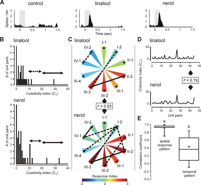
In the insect antennal lobe, odor discrimination depends on the ability of the brain to read neural activity patterns across arrays of uniquely identifiable olfactory glomeruli. Less is understood about the complex temporal dynamics and interglomerular interactions that underlie these spatial patterns. Using neural-ensemble recording, we show that the evoked firing patterns within and between groups of glomeruli are odor dependent and organized in both space and time. Simultaneous recordings from up to 15 units per ensemble were obtained from four zones of glomerular neuropil in response to four classes of odorants: pheromones, monoterpenoids, aromatics, and aliphatics. Each odor class evoked a different pattern of excitation and inhibition across recording zones. The excitatory response field for each class was spatially defined, but inhibitory activity was spread across the antennal lobe, reflecting a center-surround organization. Some chemically related odorants were not easily distinguished by their spatial patterns, but each odorant evoked transient synchronous firing across a uniquely different subset of ensemble units. Examination of 535 cell pairs revealed a strong relationship between their recording positions, temporal correlations, and similarity of odor response profiles. These findings provide the first definitive support for a nested architecture in the insect olfactory system that uses both spatial and temporal coordination of firing to encode chemosensory signals. The spatial extent of the representation is defined by a stereotyped focus of glomerular activity for each odorant class, whereas the transient temporal correlations embedded within the ensemble provide a second coding dimension that can facilitate discrimination between chemically similar volatiles.

Figure 1.

The panel of olfactory stimuli. A, Four major odorant classes, conspecific sex pheromone components (Kaissling et al., 1989) or host plant volatiles for M. sexta (Fraser et al., 2003), were used: aliphatic aldehydes (AA): nonanal and E-2-hexenal; aromatics (AR): phenylacetaldehyde and methyl salicylate; monoterpenoids (MO): (±) linalool, nerol, ocimene, myrcene, and geraniol; pheromonal components (PH): E, Z-10, 12-hexadecadienal, E, Z-11, 13-pentadecadienal [a stable mimic of the second major pheromone component (Kaissling et al., 1989)], and the blend of bal and C15. Another tested volatile that is not naturally occurring but that Manduca can learn to associate with sucrose reinforcement is the simple ketone (SK) cyclohexanone. B, Percentage of units that exhibited selective responses to MO, AA, AR, or PH volatiles and nonselective responses to two or more of these stimulus classes.

Figure 2.

Positioning the recording array in the moth AL. A, The 16 channel MRA has four shanks with four electrodes spaced evenly along each shank. The dimensions of the MRA were selected so that each shank would record activity in one of four broad zones (I-IV) of processing neuropil in the AL. B, The MRAs were placed in the same zonal arrangement in the AL from animal to animal. B1, The antennal nerve (AN) was used as a landmark to help align the MRA in the AL; the leftmost shank was always inserted into the MGC. B2, A single optical section from a confocal stack showing the lesions (white arrows) left by the four shanks of the MRA. In a different preparation, a section near the AL surface (B3) and one 25 μm deeper (B4) show the trajectories of the shanks where they penetrated through the AL neuropil. A comparison of plates 2 and 4 illustrates the variation across animals in positioning the MRA shanks, showing that the shanks can be placed repeatedly within the same AL zones, as schematized in A.

Figure 3.

Ensemble responses to brief and repeated odor pulses. Consecutive pulses of (±) linalool (time course shown at the bottom) evoked a reproducible spatial pattern of activity across a subset of units in each AL ensemble. The ensemble representation is shown as raster plots from 11 units distributed across the AL. Unit responses, as judged from their PSTHs and the CUMSUM test (±95% confidence limits), are marked according to response polarity: +, excitatory responses; -, inhibitory responses. The rate histogram (bin size, 10 msec) for unit III-1 in the bottom panel illustrates how the firing rate is modulated transiently and reproducibly by each 200 msec stimulus pulse.

Figure 4.

Conditional response probabilities. Units that responded to one member of an odor class were likely to show similar responses to other members of the same class. The color matrix summarizes the conditional response probabilities calculated for all units in the data set (n = 118). The diagonal of the matrix shows the conditional probability (p = 1.0) for each stimulus against itself. Note the separation of the data into two clusters: one for plant odorants (dashed outline) and another for pheromones (solid outline). Units that responded to monoterpenes (MO) showed the least variation across odorants. The conditional response probabilities for all units responsive to nal are outlined in black. The other stimulus compounds with strong response probabilities (p > 0.6) are indicated by asterisks. AR, Aromatics; AA, aliphatic aldehydes; PH, pheromonal components.

Figure 5.

Ensemble representations in space. A, Spatial distribution of activity evoked across the AL in one ensemble, summarizing the population response to a diverse set of odorants. The top plots show the averaged spike waveforms from two (shank I) or three (shanks II-IV) units recorded simultaneously. All units were visible on adjacent recording sites (X and Y), thus providing geometric information about the spatial origin of the signals. The bottom plot is the color-coded response matrix from the 11 unit ensemble recorded across all shanks (columns) after stimulation with the different odorants (rows). Four major stimulus classes were tested: aromatics (AR) (met, paa), aliphatic aldehydes (AA) (nal, t2h), monoterpenoids (MO) (myr, ner, oci, lin), and pheromones (PH) (c15, bal, bld), plus a simple ketone (SK) (cyc). Weak or null responses are not shown. Only the excitatory responses with an RI ≥ 2.0 SDs and inhibitory responses with an RI ≤ -2.0 SDs are shown for clarity (see color scale shown at the top of B). Note the correspondence between each stimulus category and the spatial distribution of odor-evoked activity. B, Summary of the spatial mapping of excitatory and inhibitory responses for the entire data set (n = 118 units). For excitatory responses, sex pheromone was heavily represented in zone I (MGC; red outline), aromatics were heavily represented in zone IV (blue outline), aliphatics were heavily represented in zone II (green outline), and monoterpenoids were heavily represented in zones II and III (yellow outline). In contrast to the focal organization of the excitatory response fields, inhibitory responses were distributed across the AL.

Figure 6.

Ensemble representations in time. A, B, Two of the nine units in this ensemble were easily distinguishable by spike shape [the top traces show the averaged waveforms (±SD) recorded on the 4 adjacent sites of shank II]. Although their spike shapes were different, the stimulus-response profiles of these two units were very similar. Spiking in both units (PSTHs) was increased by three monoterpenoids (lin, ner, and ger) but suppressed by the others seven stimulus compounds. C, D, To quantify the variability across responses, a color-coded correlation matrix or signature response profile was generated for each unit. Each matrix reflects the response variation between every pair of volatiles in the entire stimulus panel and thus serves as a signature of all of the responses of a single unit to the same panel of stimuli. This analysis revealed complex patterns of both high (warm colors) and low (cool colors) correlations between responses. The greatest correlations between excitatory responses (solid circles) and inhibitory responses (dashed circles) are indicated. Note also that the matrices for these two units are nearly identical, leading to a high PSI between the two units (see Materials and Methods and F). E, Cross-correlation analysis (5 msec bin width) also revealed a strong temporal relationship between these two units. The linalool-evoked correlation after trial shuffling to correct for the elevated firing rate is shown (see Materials and Methods). Interspike interval histograms for the two units are shown in the inset (y-axis, counts at each interval). F, The PSI was defined as the correlation coefficient between the response profile vectors for a pair of units (as in C and D). The exponential curve illustrates the relationship between response similarity and unit coactivity (C_%) for all pairs of units in the ensemble. For all 36 pairwise combinations, the PSI ranged from 0.24 to 0.90, revealing that pairs of units that responded similarly across the stimulus set were also positively correlated in time. The strongest relationship was found between the two units described in C and D (arrow). The coefficient of determination (r²) indicates that 37% of the total variation can be explained by this relationship. See Figure 7 for pooled data from all ensembles (n = 535 unit pairs).

Figure 7.

Relationship between profile similarity (PSI) and coactivity (C_%) across all units in all ensembles. Temporal correlations were quantified for each pair of units within each ensemble using Equation 3 to calculate C_%, the shuffle-corrected coactivity index based on the percentage of coincident spikes of the total spike count (see Materials and Methods). A, Histogram showing the distribution of C_% values for the responses of all unit pairs across all odorants (n = 5464). The inset highlights the distribution of C_% values ≥20%. B, Relationship between the PSI and C_% based on population data (n = 535 unit pairs) for all responses to lin. The series of histograms from the bottom to the top shows profile similarity distributions for progressively greater values of C_% (≥2 to ≥20%) calculated for all pairs of units. Arrows indicate mean values. C, Relationship between mean the PSI and C_% calculated for all odorants in the stimulus set. The linalool curve is shown as a thick line. D, PSI versus C_% relationships for each pair of unit responses to all odorants, separated according to intershank distance between recording sites. Odor-evoked transient synchrony occurred both within and across recording zones, with the greatest number of correlations occurring between units in adjacent zones (i.e., recording shanks separated by 125 μm).

Figure 8.

Integrating olfactory information in space and time. In this ensemble, the spatial patterns of population activity evoked by two similar stimulus compounds showed substantial overlap, but a distinct pattern of coincident firing embedded within the spatial pattern may further help distinguish one stimulus from another. A, In this unit (II-2), a 200 msec pulse (gray bar) of the monoterpenoid lin (middle), but not a control stimulus (left), evoked a brief burst of firing for each stimulus pulse. The monoterpenoid ner (right) evoked a response similar to the lin response. B, The index of coactivity (C_%) evoked by lin (top) and ner (bottom) was calculated for all possible pairs of units in this ensemble (n = 45). The frequency distributions for pairs with C_% values above (solid line) and below (dashed line) 20% are shown. Notice that the index of coactivity for the majority of pairs was ≤5%. C, Comparing spatial response patterns with coactivity patterns. The spatial response pattern for the entire ensemble is represented as a circular matrix in which individual units are ordered in a clockwise direction starting from the 12:00 position (unit I-1). Each unit is represented as a wedge around the perimeter of the matrix, and its RI is represented by the wedge color (see color scale). Also shown are the coactivity patterns (solid and dashed lines connecting unit pairs) that underlie the ensemble response to each stimulus. Note that many units showed no statistical increase in firing relative to the control response. Each connecting line represents the coactivity measure (C_%) between a specific pair of units. The spatial response patterns evoked by lin and ner are nearly identical (r = 0.93), but the coactivity patterns produced by these two odorants are distinctly different, with three pairs of units showing strong interactions in response to lin and a partially overlapping but distinct subset of seven unit pairs that showed correlations in response to ner. D, To quantify this difference, we converted the C_% values for lin and ner responses for all unit pairs (n = 45) into two vectors and then calculated the correlation coefficient between the vectors, revealing an r value for the temporal correlation that was 15% lower than that for the spatial correlation. E, The same type of correlation analysis was performed across all animals (n = 12) to determine whether the observed relationship between spatial and temporal patterning may represent a general phenomenon. The first box chart compares the similarity between the response patterns evoked by lin and ner in terms of spatial patterning only. The high r value indicates that these patterns are very similar and therefore difficult to distinguish. The second chart describes the similarity in temporal patterning after shuffle correction to account for coincident events that may be attributable only to elevated firing rates (see Materials and Methods). Each box chart shows the entire data range (error bars, 5th and 95th percentiles; horizontal lines, 25th, 50th, and 75th percentiles; filled square, mean). The results indicate that although the spatial response patterns evoked by lin and ner are highly similar across all ensembles, the coactivity patterns representing these two odor stimuli provide a greater measure of discrimination (differences are statistically significant; p < 0.05; Mann-Whitney U test; n = 535 unit pairs).

References

1. Adrian ED (1942) Olfactory reactions in the brain of the hedgehog. J Physiol (Lond) 100: 459-473. - PMC - PubMed
1. Aertsen AMHJ, Gerstein GL, Habib M, Palm G (1989) Dynamics of neuronal firing correlation: modulation of “effective connectivity.” J Neurophysiol 61: 900-917. - PubMed
1. Aungst JL, Heyward PM, Puche AC, Karnup SV, Hayar A, Szabo G, Shipley MT (2003) Centre-surround inhibition among olfactory bulb glomeruli. Nature 426: 623-629. - PubMed
1. Brown EN, Kass RE, Mitra PP (2004) Multiple neural spike train data analysis: state-of-the-art and future challenges. Nat Neurosci 7: 456-461. - PubMed
1. Buonviso N, Chaput MA (1990) Response similarity to odors in olfactory bulb output cells presumed to be connected to the same glomerulus: electrophysiological study using simultaneous single unit recordings. J Neurophysiol 63: 447-454. - PubMed
Publication types