Evaluating concentration estimation errors in ELISA microarray experiments

Abstract

Background: Enzyme-linked immunosorbent assay (ELISA) is a standard immunoassay to estimate a protein's concentration in a sample. Deploying ELISA in a microarray format permits simultaneous estimation of the concentrations of numerous proteins in a small sample. These estimates, however, are uncertain due to processing error and biological variability. Evaluating estimation error is critical to interpreting biological significance and improving the ELISA microarray process. Estimation error evaluation must be automated to realize a reliable high-throughput ELISA microarray system. In this paper, we present a statistical method based on propagation of error to evaluate concentration estimation errors in the ELISA microarray process. Although propagation of error is central to this method and the focus of this paper, it is most effective only when comparable data are available. Therefore, we briefly discuss the roles of experimental design, data screening, normalization, and statistical diagnostics when evaluating ELISA microarray concentration estimation errors.

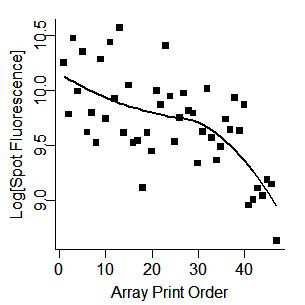
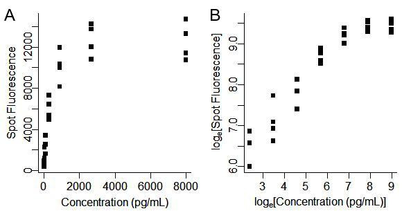
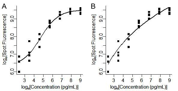
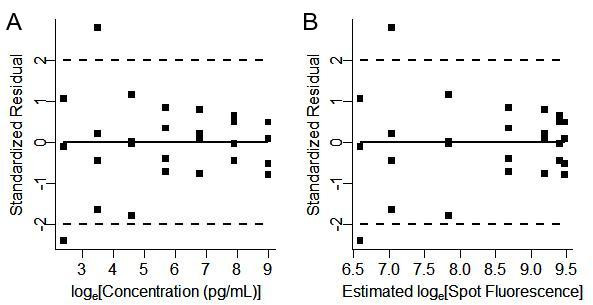
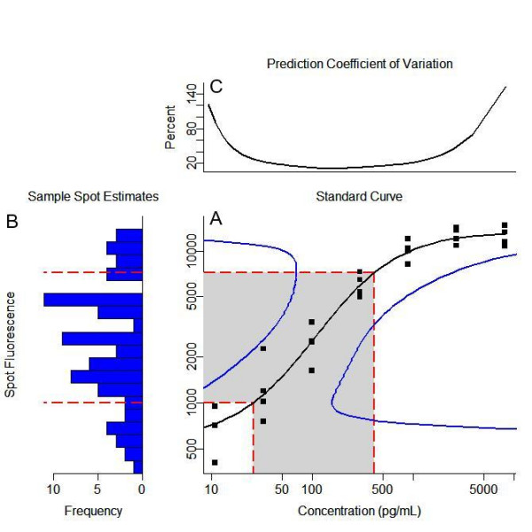
Results: We use an ELISA microarray investigation of breast cancer biomarkers to illustrate the evaluation of concentration estimation errors. The illustration begins with a description of the design and resulting data, followed by a brief discussion of data screening and normalization. In our illustration, we fit a standard curve to the screened and normalized data, review the modeling diagnostics, and apply propagation of error. We summarize the results with a simple, three-panel diagnostic visualization featuring a scatterplot of the standard data with logistic standard curve and 95% confidence intervals, an annotated histogram of sample measurements, and a plot of the 95% concentration coefficient of variation, or relative error, as a function of concentration.

Conclusions: This statistical method should be of value in the rapid evaluation and quality control of high-throughput ELISA microarray analyses. Applying propagation of error to a variety of ELISA microarray concentration estimation models is straightforward. Displaying the results in the three-panel layout succinctly summarizes both the standard and sample data while providing an informative critique of applicability of the fitted model, the uncertainty in concentration estimates, and the quality of both the experiment and the ELISA microarray process.

Figure 1

Control spot fluorescence and slide print order We expect control spot intensity to be constant across slide print order. The trend, estimated with loess regression, indicates a processing effect due to printing order. In this case, the decrease in control spot intensity, coupled with knowledge of the printing process, suggests that the quantity of printed material is decreasing over a printing run.

Figure 2

Spot fluorescence and standard concentration A graph of spot fluorescence as a function of standard concentration (A) shows that both the difference in concentration and the variability in spot fluorescence increase with concentration. Both negatively affect model fitting and subsequent statistical inferences due to the excessive leverage of the larger concentrations and the heteroskedasticity of the spot intensities. In this case, log_e transforms of both concentration and spot fluorescence reduce the excessive leverage and improve the homogeneity (B). The log transformation is consistent with the featured concentration dilution series and is a common transformation of chemical measurements that often are assumed log normally distributed.

Figure 3

Candidate standard curves A review of the graphs of a four-parameter logistic curve (A) and a power law curve (B) suggests that the former shows higher fidelity to the data and is a better choice for the standard curve in this case.

Figure 4

Modeling diagnostics The points in graphs of the standardized residuals versus the log_e standard concentrations (A) and the standardized residuals versus the estimated log_e spot intensities (B) are reasonably well behaved, showing no strong systematic trends or deviations from the zero line. These indicate that the four-parameter logistic model is acceptable, that subsequent statistical inferences are reasonable, but that a better model may exist in another model family.

Figure 5

Three-panel diagnostic summary The standard curve panel (A) of the three-panel diagnostic summary features a scatterplot of the data, the estimated standard curve (black line), the 95% confidence intervals (blue lines), and the region of acceptable errors (grey). For this example, the acceptable segment of the standard curve (i.e., the segment with concentration estimation errors acceptable to us) covers spot intensities from about 1000 to 7500 intensity units and concentrations from about 25 to 500 pg/ml. The histogram of sample intensities (B) suggests that about one-fifth of the sample spot intensities is below the detection limit of about 1000 units, about three-fifths will produce estimated concentrations in the acceptable range, and one-fifth exceeds the acceptable range. With regard to remeasuring the standards in this experiment or imaging in future experiments, the three-panel graph suggests that it may be worthwhile to attempt to extend the acceptable range. It also suggests that the normalization between the standards measurements and sample measurements should be revisited. The graph of the concentration coefficient of variation as function of concentration (C) offers an alternative summary of the estimation errors over the range of concentrations.

References

-
- Varnum SM, Woodbury RL, Zangar RC. A protein microarray ELISA for screening biological fluids. Methods Mol Biol. 2004;264:161–172. - PubMed
- Racine-Poon A, Weihs C, Smith AFM. Estimation of relative potency with sequential dilution errors in radioim-munoassay. Biometrics. 1991;47:1235–1246. - PubMed
- Giltinan DM, Davidian M. Assays for recombinant proteins: a problem in non-linear calibration. Statistics in Medicine. 1994;13:1165–1179. - PubMed
Publication types
MeSH terms
Substances
LinkOut - more resources
Full Text Sources
Other Literature Sources