Evolution of recombination due to random drift

Abstract

In finite populations subject to selection, genetic drift generates negative linkage disequilibrium, on average, even if selection acts independently (i.e., multiplicatively) upon all loci. Negative disequilibrium reduces the variance in fitness and hence, by Fisher's (1930) fundamental theorem, slows the rate of increase in mean fitness. Modifiers that increase recombination eliminate the negative disequilibria that impede selection and consequently increase in frequency by "hitchhiking." Thus, stochastic fluctuations in linkage disequilibrium in finite populations favor the evolution of increased rates of recombination, even in the absence of epistatic interactions among loci and even when disequilibrium is initially absent. The method developed within this article allows us to quantify the strength of selection acting on a modifier allele that increases recombination in a finite population. The analysis indicates that stochastically generated linkage disequilibria do select for increased recombination, a result that is confirmed by Monte Carlo simulations. Selection for a modifier that increases recombination is highest when linkage among loci is tight, when beneficial alleles rise from low to high frequency, and when the population size is small.

Figure 1.—

Allele frequency change in a finite population. The thick curve shows the average frequency over time of the allele P_j, with selective advantage s_j = 0.1 and initial frequency p_j0 = 0.01, in a population of size 2N = 10,000, using Equation 4a to determine the departure from the deterministic trajectory (p_j/q_j = e^sjtp_j0/q_j0). Although drift causes P_j to rise less rapidly on average than expected in an infinitely large population, the effect is small, shifting the trajectory to the right by an amount approximately equal to the thickness of the curve. We therefore use the deterministic trajectory to approximate p_j throughout this article, which is a reasonable assumption provided that Ns_j ≫ 1. The thin curves show the expected allele frequency ±2 standard deviations based on (4b) (a weak selection approximation generates indistinguishable results and is not shown). Dots show simulation results for the mean allele frequency ±2 standard deviations, based on 1,000,000 replicates.

Figure 2.—

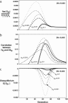
Effects of drift and selection on disequilibrium in a finite population under directional selection. (a) Variance in disequilibrium scaled to p_jq_jp_kq_k; (b) correlation between effects of drift on allele frequency and on disequilibrium (Corr[δp_jδD_jk]); (c) average disequilibrium over time. In each case, the initial allele frequencies are p_j0 = p_k0 = 0.001 (dotted curves), 0.01 (dashed curves), or 0.1 (solid curves), where the latter curves are shifted to the right by 23.1 and 47.1 generations, respectively, so that allele frequencies are equivalent for all curves at any point in time. The thick curves give the exact calculations from (5), while the thin curves show the weak selection approximation (B5). Results are shown for s_j = s_k = 0.1, r_jk = 0.1, and 2N = 10,000.

Figure 3.—

Observed and expected disequilibrium under directional selection. The disequilibria expected from (5) (curves) and observed in simulations with 1,000,000 replicates (dots, with bars indicating ±2 standard errors) are shown for (a) 2N = 10,000 and (b) 2N = 100,000. Equation 5 accurately estimates the amount of disequilibrium generated except when there are only 10 initial copies of each allele (p_j0 = p_k0 = 0.001 and 2N = 10,000). Otherwise, the disequilibrium scales directly with 1/(2N). With only 10 copies initially, both beneficial alleles did not always fix, and we report only the disequilibrium observed in those cases in which both beneficial alleles remain. Remaining parameters and symbols are as in Figure 2.

Figure 4.—

The most extreme value of the average disequilibrium under directional selection, plotted on a log-log scale. During the spread of beneficial alleles, the expected disequilibrium from (5) (thick curves) becomes negative, taking on the minimum values shown. More extreme disequilibria are observed when the initial allele frequencies are low [compare p_j0 = p_k0 = 0.01 (dashed curves) to p_j0 = p_k0 = 0.1 (solid curves)] and when recombination is rare, in which case the expected disequilibrium approaches the minimum value that D_jk may take (−0.25, corresponding to the bottom axis of the graph). The thin curve gives the most extreme value of the disequilibrium from the QLE approximation (B3c), which is accurate only when r_jk > 0.1. Dots show the most extreme value of the mean disequilibrium observed in 1,000,000 replicate simulations for r_jk = 0.001, 0.01, and 0.1. X's represent a numerical evaluation of the weak selection approximation, (B5c). Remaining parameters and symbols are as in Figure 2.

Figure 5.—

The influence of the relative position of the modifier, α = r_ik/r_jk, on g(α). According to the QLE approximation (7), the change in frequency of a modifier is proportional to g(α) (solid curve) when recombination rates are small but larger than the selection coefficients. The dashed curve compares this approximation to the full QLE result [the complicated function f(r) in (S2.4) with no interference], which applies even when recombination rates are high.

Figure 6.—

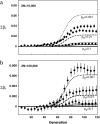
The cumulative selection gradient, ∑β_i, on a modifier of recombination as a function of time under directional selection for (a) 2N = 10,000 and (b) 2N = 100,000. The selection gradient per generation, β_i, is given by the rise in these curves over a single generation. Equations 2 and 3 are used to generate the curves for p_j0 = p_k0 = 0.001 (dotted curves), 0.01 (dashed curves), and 0.1 (thick solid curves), where the latter two are shifted to the right as in Figure 2. Simulations (dots) are based on 10,000,000 replicates for a modifier that changes recombination by δr_j,k|i = 0.05 and that starts at frequency p_i0 = 0.5. With p_j0 = p_k0 = 0.001 and 2N = 10,000, both alleles did not always fix, and we report changes in the modifier frequency conditional on fixation. The QLE prediction (S2.4) is shown as a thin solid curve and fails to account for the sensitivity to initial allele frequencies when recombination is not large relative to selection. Remaining parameters are s_j = s_k = 0.1 and r_ij = r_jk = 0.1, with gene order ijk and no crossover interference.

Figure 7.—

The net selection gradient, β_i,net, on a modifier of recombination as a function of the recombination rates under directional selection, plotted on a log-log scale. Equations 2 and 3 are used to generate the thick curves for r_ij = 0.01, 0.1, and 0.5 (from top to bottom). The thin curves give the net change in modifier frequency using the QLE approximation (S2.4) for the same range of r_ij. Dots show simulation results based on 1,000,000 replicates for r_jk = 0.001, 0.01, and 0.1 and r_ij = 0.01 and 0.1 (from top to bottom; standard errors were too large for r_ij = 0.5 to assess the effect). In the simulations, the modifier changes recombination by an amount δr_j,k|i = r_jk/2 and starts at frequency p_i0 = 0.5. The gene order is ijk, and there is no interference. Remaining parameters are s_j = s_k = 0.1, p_j0 = p_k0 = 0.01, and 2N = 10,000, with gene order ijk and no crossover interference.

Figure 8.—

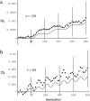
The cumulative selection gradient, ∑β_i, on a modifier of recombination under fluctuating selection. The strength of selection on loci j and k varies sinusoidally over time, with the maximum strength of selection set to α_j = α_k = 0.1 and with both loci in phase. The gene order is ijk, there is no interference, and δr_j,k|i = r_jk/2. Equations 2 and 3 are used to generate the expected change in the modifier (solid curves) starting with p_i0 = p_j0 = p_k0 = 0.5 in a population of size 2N = 100,000. Dots show simulation results based on 20,000,000 replicates (±2 standard errors). (a) Period (τ) is 120 generations, r_jk = 0.1, and r_ij = 0.1. (b) Period (τ) is 60 generations, r_jk = 0.02, and r_ij = 0.01.

Figure 9.—

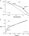
The selection gradient on a modifier of recombination multiplied by the population size, 2Nβ_i, at steady state under sinusoidal selection, plotted on a log-log scale. The x-axis is the recombination rate between adjacent loci, assumed to lie in the order ijk, with r = r_ij = r_jk. The thick curve illustrates the predicted change in the modifier from iteration of (2) and (3). The thin solid curve illustrates (8), which is a low-recombination approximation to the recursion equations. The long dashed curve illustrates the QLE solution (S2.4). The dot marks the simulation result reported in Figure 8a. Parameter values were set to α_j = α_k = 0.1, p_j0 = p_k0 = 0.5, with (a) period τ = 120 across a range of recombination rates and (b) a range of periods, τ, with rτ = α = 0.1. The per generation change in the modifier (thick curves) is much higher when the period of fluctuating selection is longer; in this case, alleles pass through both low and high frequency within each period, increasing the fluctuations in disequilibrium that drive selection for the modifier.

References

1. Altenberg, L., and M. W. Feldman, 1987. Selection, generalized transmission and the evolution of modifier genes. I. The reduction principle. Genetics 117: 559–572. - PMC - PubMed
1. Barton, N. H., 1995. a A general model for the evolution of recombination. Genet. Res. 65: 123–144. - PubMed
1. Barton, N. H., 1995. b Linkage and the limits to natural selection. Genetics 140: 821–841. - PMC - PubMed
1. Barton, N. H., 1998. The effect of hitch-hiking on neutral genealogies. Genet. Res. 72: 123–133.
1. Barton, N. H., 2000. Genetic hitchhiking. Philos. Trans. R. Soc. Lond. B 355: 1553–1562. - PMC - PubMed
Publication types