

Phenotypic error threshold; additivity and epistasis in RNA evolution
- PMID: 15691379
- PMCID: PMC550645
- DOI: 10.1186/1471-2148-5-9
Phenotypic error threshold; additivity and epistasis in RNA evolution
Abstract
Background: The error threshold puts a limit on the amount of information maintainable in Darwinian evolution. The error threshold was first formulated in terms of genotypes. However, if a genotype-phenotype map involves redundancy ("mutational neutrality"), the error threshold should be formulated in terms of phenotypes since there is no unique fittest genotype. A previous study formulated the error threshold in terms of phenotypes, and their results showed that a rather low degree of mutational neutrality can increase the error threshold unlimitedly.
Results: We obtain an analytical formulation of the phenotypic error threshold by considering the "additive assumption", in which base substitutions do not influence each other (no epistasis). Our formulation shows that an increase of the error threshold due to mutational neutrality is limited. Computer simulations of RNA evolution are conducted to verify our formulation, and the results show a good agreement between the analytical prediction and the simulations. The comparison with the previous formulation illustrates that it is important for the prediction of the error threshold to consider that the number of base substitutions per replication is rather large near the error threshold. To examine the additive assumption, a detailed analysis of additivity and epistasis in RNA folding of a particular sequence is performed. The results show a high degree of epistasis in RNA folding; furthermore, the analysis also elucidates the reason of the success of the additive assumption.
Conclusions: We conclude that an increase of the error threshold by mutational neutrality is limited, and that the additive assumption achieves a good prediction of the error threshold in spite of a high degree of epistasis in RNA folding because the average number of base substitutions of sequences retaining the phenotype per replication is sufficiently small to avoid of the effect of epistasis.
Figures
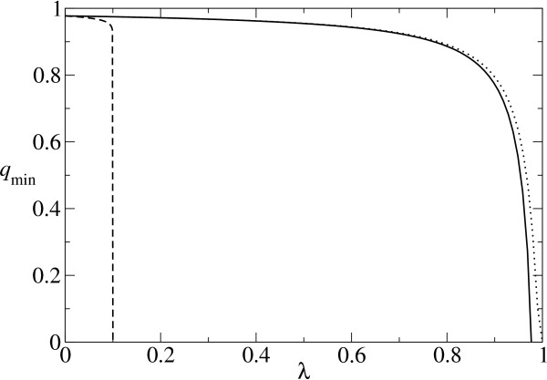
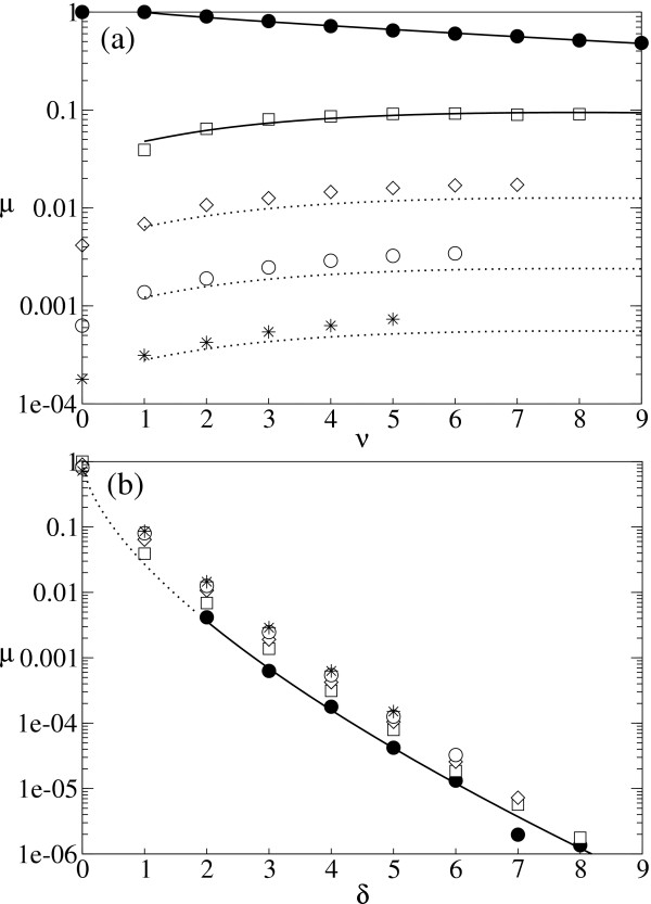
 . The dotted line represents the so calculated error threshold in this extreme example. The x-axis for the dotted line (i.e., λ) is calculated as (N - Nδ)/N. The dashed line is obtained from the formulation of Reidys et al. [5] (Eq. 5). In all cases, N = 100 and σ = 10. (The same values of N and of σ as those used in [5] are chosen for a comparison purpose.)
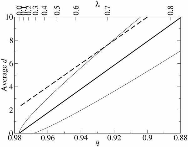
 . The dashed line represents the average d per replication, which is N(1 - qmin). N is 100 and σ is 10. The lines are plotted against qmin (the lower x-axis), and the corresponding λ is shown in the upper x-axis.
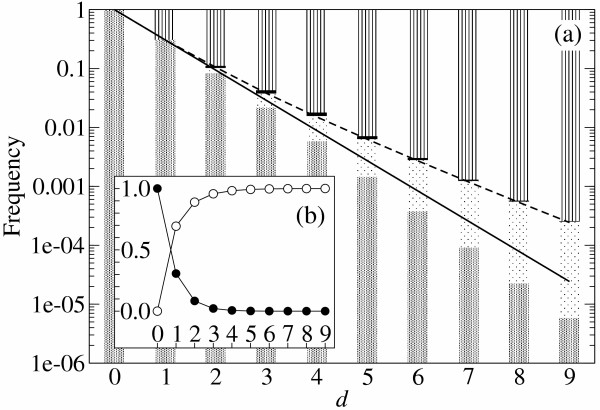
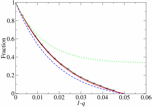
 (d), see Methods section – Probabilistic approach). (b) Linear plot. Symbols: ● the frequency of the neutral mutants (additive neutral and positive epistasis); ○ the frequency of the deleterious mutants (additive deleterious and negative epistasis).
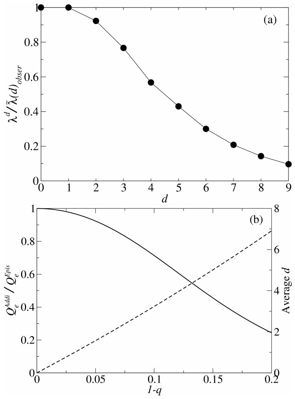
Similar articles
-
Error thresholds in genetic algorithms.Evol Comput. 2006 Summer;14(2):157-82. doi: 10.1162/evco.2006.14.2.157. Evol Comput. 2006. PMID: 16831105
-
Agent-based model of genotype editing.Evol Comput. 2007 Fall;15(3):253-89. doi: 10.1162/evco.2007.15.3.253. Evol Comput. 2007. PMID: 17705779
-
Determinants of simulated RNA evolution.J Theor Biol. 2006 Feb 7;238(3):726-35. doi: 10.1016/j.jtbi.2005.06.019. Epub 2005 Aug 11. J Theor Biol. 2006. PMID: 16098538
-
Evolution in silico and in vitro: the RNA model.Biol Chem. 2001 Sep;382(9):1301-14. doi: 10.1515/BC.2001.162. Biol Chem. 2001. PMID: 11688713 Review.
-
Perspectives on protein evolution from simple exact models.Appl Bioinformatics. 2002;1(3):121-44. Appl Bioinformatics. 2002. PMID: 15130840 Review.
Cited by
-
Less can be more: RNA-adapters may enhance coding capacity of replicators.PLoS One. 2012;7(1):e29952. doi: 10.1371/journal.pone.0029952. Epub 2012 Jan 23. PLoS One. 2012. PMID: 22291898 Free PMC article.
-
The origin of replicators and reproducers.Philos Trans R Soc Lond B Biol Sci. 2006 Oct 29;361(1474):1761-76. doi: 10.1098/rstb.2006.1912. Philos Trans R Soc Lond B Biol Sci. 2006. PMID: 17008217 Free PMC article.
-
Modular evolution and increase of functional complexity in replicating RNA molecules.RNA. 2007 Jan;13(1):97-107. doi: 10.1261/rna.203006. Epub 2006 Nov 14. RNA. 2007. PMID: 17105993 Free PMC article.
-
The role of complex formation and deleterious mutations for the stability of RNA-like replicator systems.J Mol Evol. 2007 Dec;65(6):668-86. doi: 10.1007/s00239-007-9044-6. Epub 2007 Oct 23. J Mol Evol. 2007. PMID: 17955153
-
Pathways to extinction: beyond the error threshold.Philos Trans R Soc Lond B Biol Sci. 2010 Jun 27;365(1548):1943-52. doi: 10.1098/rstb.2010.0076. Philos Trans R Soc Lond B Biol Sci. 2010. PMID: 20478889 Free PMC article.
References
-
- Maynard Smith J, Szathmary E. The Major Transitions in Evolution. reprint. New York: Oxford University Press; 1997. Chaper 4; pp. 41–58.
MeSH terms
Substances
LinkOut - more resources
Full Text Sources
