A molecular-mechanical model of the microtubule

Abstract

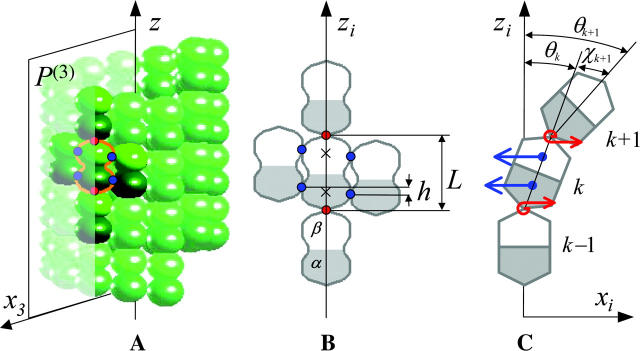
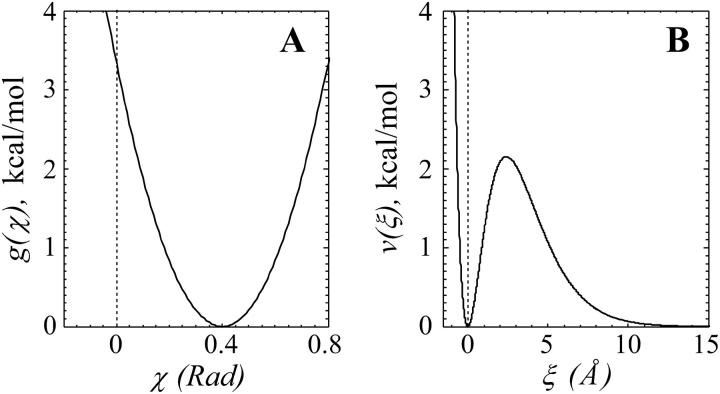
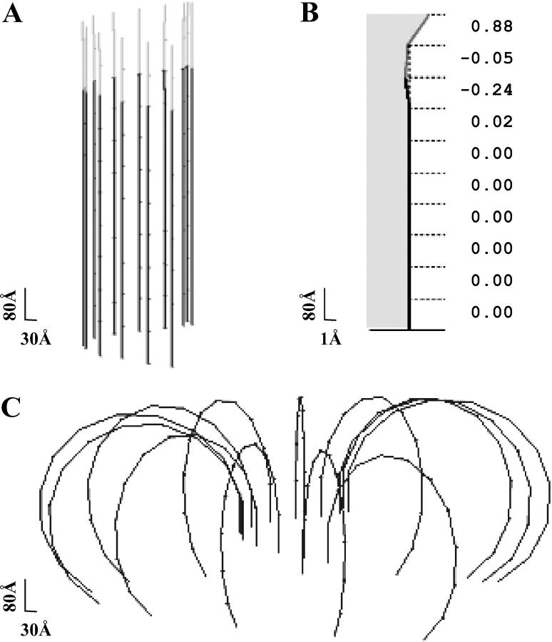
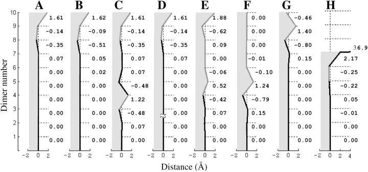
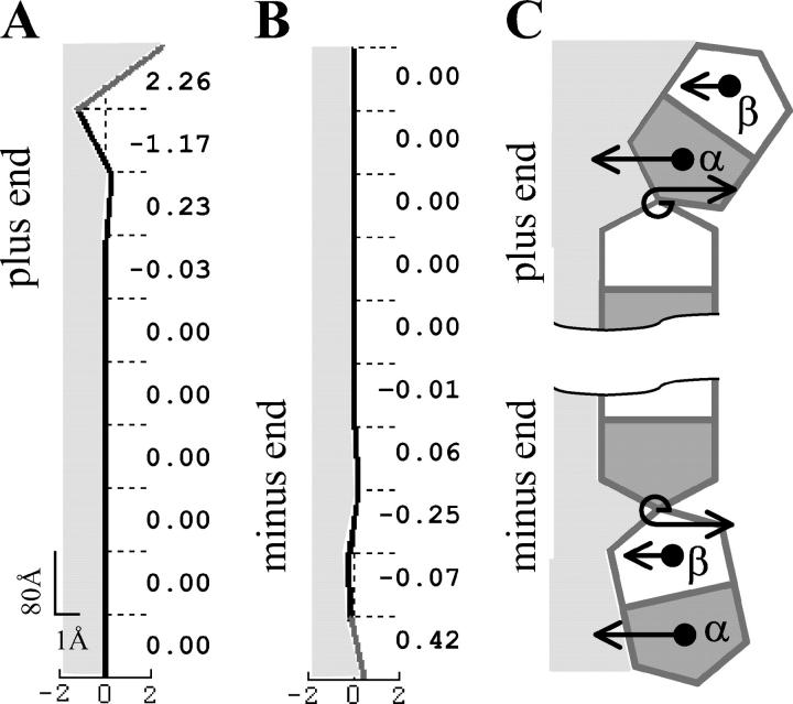
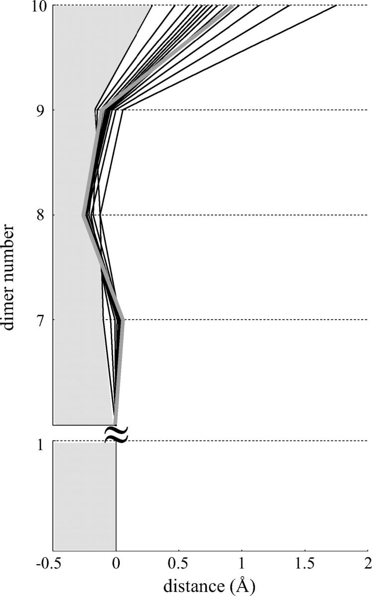
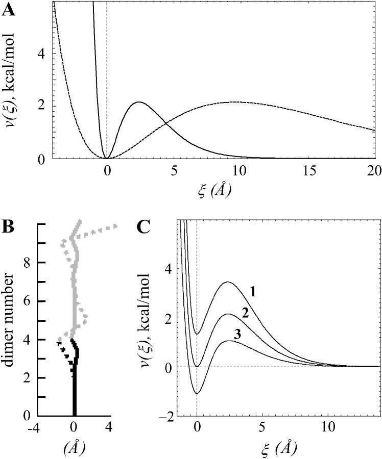
Dynamic instability of MTs is thought to be regulated by biochemical transformations within tubulin dimers that are coupled to the hydrolysis of bound GTP. Structural studies of nucleotide-bound tubulin dimers have recently provided a concrete basis for understanding how these transformations may contribute to MT dynamic instability. To analyze these ideas, we have developed a molecular-mechanical model in which structural and biochemical properties of tubulin are used to predict the shape and stability of MTs. From simple and explicit features of tubulin, we define bond energy relationships and explore the impact of their variations on integral MT properties. This modeling provides quantitative predictions about the GTP cap. It specifies important mechanical features underlying MT instability and shows that this property does not require GTP-hydrolysis to alter the strength of tubulin-tubulin bonds. The MT plus end is stabilized by at least two layers of GTP-tubulin subunits, whereas the minus end requires at least one; this and other differences between the ends are explained by asymmetric force balances. Overall, this model provides a new link between the biophysical characteristics of tubulin and the physiological behavior of MTs. It will also be useful in building a more complete description of MT dynamics and mechanics.

FIGURE 1

MT geometry and the forces acting between dimers. (A) A segment of a three-dimensional drawing of the MT polymer in a straight configuration with 13 individual PFs arranged with a helical pitch of three monomers per turn of the helix. Axis z is the central axis of the MT and points to the MT's plus end. MT dimers consist of the lower α-tubulin (dark green) and the upper β-tubulin (light green) monomers. Each nonterminal dimer (e.g., the dimer circled with an orange line) has six points of interaction with adjacent dimers (shown with darker color): longitudinal (red dots), and lateral (blue). The MT space is divided into 13 equal sectors. Plane P⁽³⁾ (shown as semitransparent) contains the third PF axis and includes the longitudinal interaction points for all dimers in this PF. (B) An enlarged schematic diagram of a dimer and its adjacent neighbors showing the positions of interaction points; z_i is the axis of the ith PF, h is a longitudinal shift between neighboring PFs, L is the dimer's length. Centers of monomers for a central dimer are shown with crosses. (C) Side view of a single bent PF in plane P⁽ⁱ⁾. Bending of each PF (exaggerated) is assumed to occur only in its respective plane P (x_i, z_i). For each dimer the angle θ describes the dimer's tilting relative to the respective PF's axis, whereas χ is the angle between a dimer and its upper neighbor. The longitudinal forces (red bent arrows) bend the PF such that all angles tend to the equilibrium The lateral forces correspond to α−α and β−β bonds and have their projections (blue straight arrows) in the plane P⁽ⁱ⁾.

FIGURE 2

Energy potentials for dimer interactions. (A) The potential function used to describe longitudinal interactions is a quadratic function of the angle χ; its minimum for GDP-dimers is at Rad (shown). The minimum for GTP-dimers is shifted closer to zero, since (not shown). Vertical broken line here and in B marks 0. (B) The potential for lateral interactions has its maximum when the distance between interaction points 2r_o = 2.4 Å; it is minimal when dimers are either not separated (r = ρ) or when r tends to infinity (the potential shown is for ρ = 0).

FIGURE 3

Steady-state MT configurations. Numerical calculations were carried out using the model of a helical MT and for a = 0.65, γ = 1, N = 10 (see Mathematical Model and Supplementary Materials for details). Black and shaded segments represent dimers in the GDP and GTP form, respectively. (A) The three-dimensional arrangement of all PFs in a MT with a 2T plus-end cap. (B) The side view of the eighth PF from the same MT as shown in A. Numbers on the right are the deviations (in angstroms) of the dimer's top interaction points from the vertical axis. Shaded area corresponds to the inner side of the MT. Note difference in scale between ordinate and abscissa. (C) The equilibrium configuration of a MT with the same parameters as in A but with no cap. Under normal conditions, after separation of lateral attachments, the dimers also loose their longitudinal connections; the PFs in C are shown bent but unbroken because in the model the longitudinal bonds do not separate. This feature does not interfere with analysis of the events occurring before the dimer's dissociation.

FIGURE 4

Side-view profiles of a single PF from nonhomogeneous MTs. The numerical calculations were carried out using the model for a nonhelical 13_0 MT with 10 tubulin layers (N = 10, except in D, where N = 20) for a = 0.65, γ = 1, and (A–E, H), or (F and G). See Fig. 3 for other details. All MTs have a 2T-cap at their plus ends except E and F, where the GTP cap has six layers, and H, where there is no cap. In B the strength of all lateral bonds for GDP-dimers was reduced 10-fold, relative to GTP-dimers. In C, the MT has the same parameters as in A, but it contains a layer of nonterminal GTP-dimers. H shows the steady-state configuration for a MT without a cap, but with a single nonterminal GTP layer. The plus end of such a MT underwent catastrophe, but PF bending (almost horizontal black line) stopped at the GDP layer above the GTP-containing dimers.

FIGURE 5

Differences between plus and minus ends. Fine structure of the plus (A) and minus (B) ends in the same 13_0 MT with 1T-cap; a = 1.25, γ = 0.1, ; a > a_cr of the plus end, so that both ends are stable when each has a 1T-cap. See legend of Fig. 1 for more details. (C) A schematic illustration of how structural differences at the ends lead to their different shapes and stabilities. The bending (not to scale) at two ends of a single PF is shown for γ < 1. Straight arrows show amplitude and direction of the lateral forces acting between the monomers in this PF and its neighbors (not shown). Round arrows correspond to the bending forces between the head-to-tail adjacent dimers in the same PF.

FIGURE 6

Fine structure of the tips of all PFs in a helical MT. The side views of all 13 PFs (black). In the first PF the dimers have neighbors for all lateral interaction points (most straight black contour), whereas the 13th PF is missing three lateral bonds (most bent black contour). Structure of the PF in a nonhelical MT with the same parameter values is shown for a comparison (thick shaded contour).

FIGURE 7

Roles of the parameters describing the potential function for the lateral bonds. (A) Two energy potential functions described by the same function (Eq. 3) but with different r_o: 1.2 Å (solid line) and 4.8 Å (dashed line). (B) The profiles of PFs for 13_0 5T-cap MT were calculated for two energy potentials shown in A. (C) Energy potential functions with the same parameters (ascending parts for 0 < ξ < 2r_o = 2.4 Å, width of the well and the barrier's height), except the levels at their minima. Curve 2 is described by Eq. 3 and is the same as shown on Fig. 2 B. Curve 1 is given by curve 3 by where A is the same as for curve 2.

References

1. Arnal, I., E. Karsenti, and A. A. Hyman. 2000. Structural transitions at microtubule ends correlate with their dynamic properties in Xenopus egg extracts. J. Cell Biol. 149:767–774. - PMC - PubMed
1. Bayley, P., M. Schilstra, and S. Martin. 1989. A lateral cap model of microtubule dynamic instability. FEBS Lett. 259:181–184. - PubMed
1. Caplow, M. 1992. Microtubule dynamics. Curr. Opin. Cell Biol. 4:58–65. - PubMed
1. Caplow, M., and L. Fee. 2003. Concerning the chemical nature of tubulin subunits that cap and stabilize microtubules. Biochemistry. 42:2122–2126. - PubMed
1. Caplow, M., and J. Shanks. 1996. Evidence that a single monolayer tubulin-GTP cap is both necessary and sufficient to stabilize microtubules. Mol. Biol. Cell. 7:663–675. - PMC - PubMed
Publication types
LinkOut - more resources