Functional architecture of retinotopy in visual association cortex of behaving monkey

Abstract

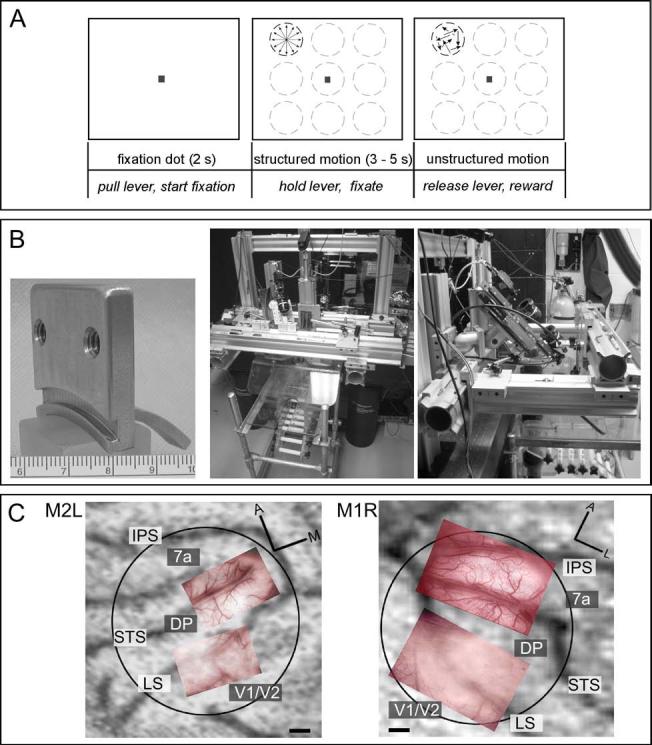
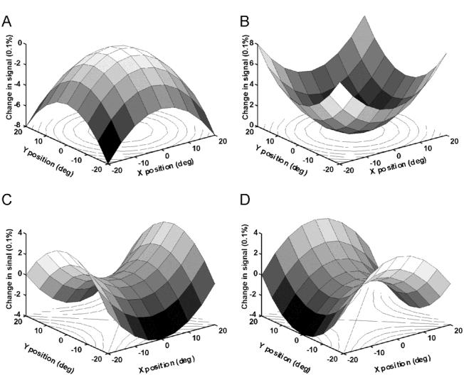
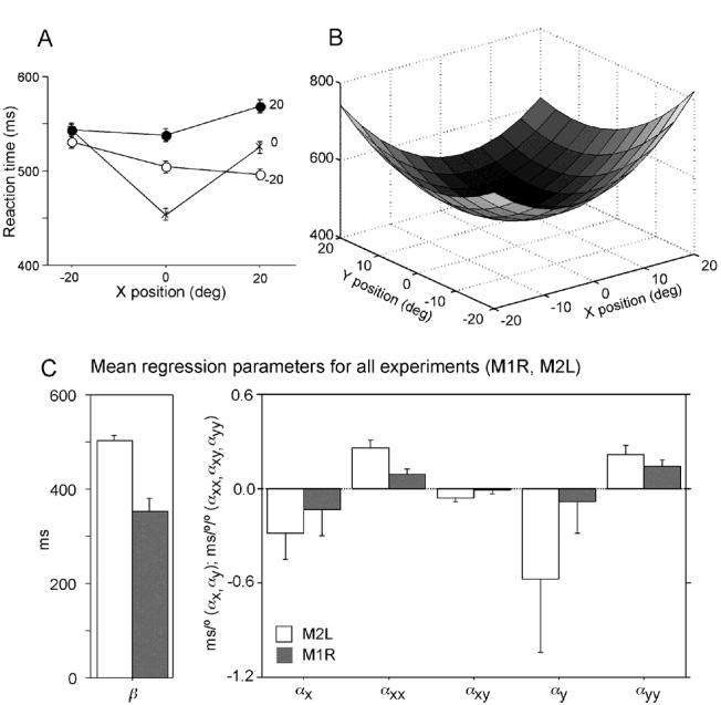
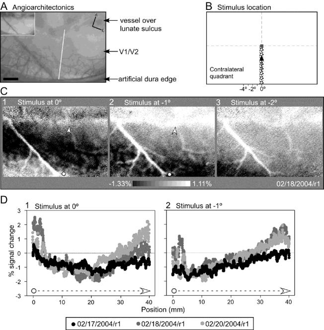
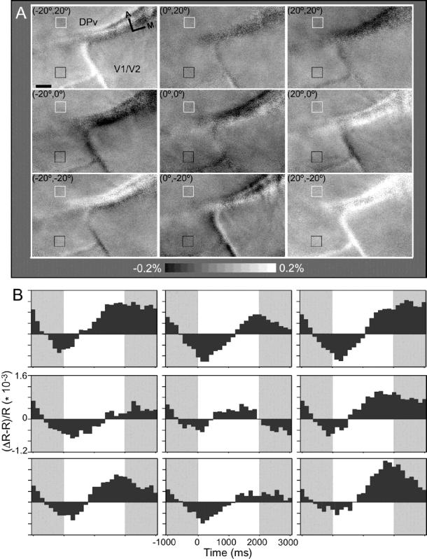
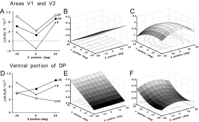
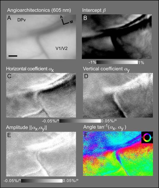
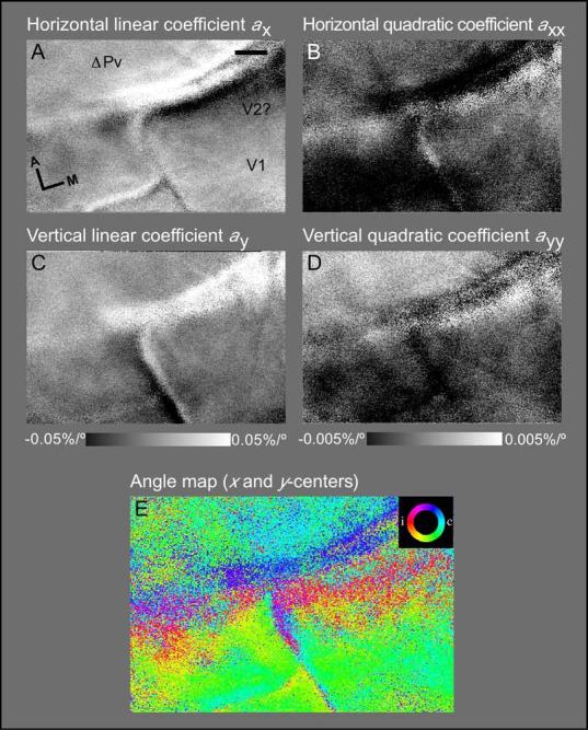
While the receptive field properties of single neurons in the inferior parietal cortex have been quantitatively described from numerous electrical measurements, the visual topography of area 7a and the adjacent dorsal prelunate area (DP) remains unknown. This lacuna may be a technical byproduct of the difficulty of reconstructing tens to hundreds of penetrations, or may be the result of varying functional retinotopic architectures. Intrinsic optical imaging, performed in behaving monkey for extended periods of time, was used to evaluate retinotopy simultaneously at multiple positions across the cortical surface. As electrical recordings through an implanted artificial dura are difficult, the measurement and quantification of retinotopy with long-term recordings was validated by imaging early visual cortex (areas V1 and V2). Retinotopic topography was found in each of the three other areas studied within a single day's experiment. However, the ventral portion of DP (DPv) had a retinotopic topography that varied from day to day, while the more dorsal aspects (DPd) exhibited consistent retinotopy. This suggests that the dorsal prelunate gyrus may consist of more than one visual area. The retinotopy of area 7a also varied from day to day. Possible mechanisms for this variability across days are discussed as well as its impact upon our understanding of the representation of extrapersonal space in the inferior parietal cortex.

Figure 1

Experimental methods. (A) Stimulus sequence. The trial starts with presentation of the fixation dot in the center of the screen that the monkey has to fixate throughout the trial until reward. The monkey needs to pull the lever back to continue the trial. The optic flow stimulus (expansion flow) is presented in one of nine locations (position −20°,20° in illustration) on the screen 2000 ms after the fixation point is on. The motion stimulus change from structured optic flow to unstructured motion occurs between 5000 and 6000 ms after fixation point onset; the monkey releases the lever for the reward. (B) Optical imaging apparatus. Left panel: close view of the stainless steel head holder. Once implanted, the lower portion, i.e., the curved grove in the front and the support extending from the back part are embedded in the cement, but does not touch the skull. The monkey's head holder is secured with two hardened steel 20-1/4” screws to a steel plate bolted to a CX-95A carrier attached to a horizontal Newport X-95 beam that provides excellent rigidity. Middle panel: a front view of the assembly on the floating air table including the primate chair in the lower portion of the image. The CCD camera and lenses are in the upper left portion of the image. The monkey's head is attached to the horizontal X-95 rail in the front. Right panel: a closer view of the camera and lens system, which are secured on a X-26 steel rail that can be slid up and down. This sliding rail in turn is attached firmly to AX-95 devices, whose angle can also be adjusted. Two Nikon 50 mm 1.2 lenses are illustrated. (C) Anatomical location of optical chambers for both monkeys (left, M2L; right, M1R) superimposed on structural MRIs. Within one chamber, two or three exposures were selected: one posterior centered over the lunate sulcus (LS), which included areas V1/V2 and DPv (lower insets with angioarchitectonic maps at 540 nm), and one anterior at the tip of the superior temporal sulcus (STS), which includes areas DP and 7a (upper insets with angioarchitectonic maps at 540 nm). In M1R, a third camera placement further posterior was used to image V1/V2 (gray rectangular frame). Scale bar, 2 mm.

Figure 2

Illustrative quadratic functions. (A) Negative quadratic coefficients (α_xx, α_yy) yield a peak, which was often found in V1/V2. (B) Positive quadratic coefficients (α_xx, α_yy) yield a valley. (C) Positive (α_xx) and negative (α_yy) coefficients yield a saddle point. (D) Negative (α_xx) and positive (α_yy) coefficients also yield a saddle point. ||α_xx||=||α_yy||=0.01%/°/°; ||α_x||=||α_y||=0%/°; β=0%, eq. 2.

Figure 3

Reaction time data. (A) Single experimental run of 482 trials for M2L (dataset 04/29/2003/gm). Mean reaction time computed for each of nine positions of the 3 × 3 grid (eccentricity 20°). The three curves (crosses, open and filled circles) represent the three different y-positions (0°,−20° and 20°, respectively). (B) Fit for the reaction time data for the experiment shown in (A). The resulting regression is RT = −0.482x − 1.962y + 0.364x² + 0.228y² + 485.6 ms. (C) Regression parameters from the stepwise regression for the reaction time data across all experiments and for both monkeys. All values given as mean ± standard error.

Figure 4

Retinotopic mapping of areas V1 and V2 with elongated thin bar stimuli in M1R. (A) Angioarchitectonics obtained at 540 nm and 605 nm (small inset) showing the large blood vessel over the lunate sulcus (LS) on the top of the image. The posterior edge of the artificial dura is visible on the bottom of the image. The white bar indicates the slice for the profile plots in (D). Scale bar, 1 mm. (B) Stimulus setup for elongated thin bar experiment. The dots move in one direction within the bar window (1° width, 12° height) that is placed at 0, −1, −2, or −3° from the lower vertical meridian (contralateral quadrant). (C) Blank-subtracted activation maps shown for three stimulus locations (C1, 0°; C2, −1°; C3, −2°). Scale of gray level range for all maps shown on the bottom of the figure. Dataset 02/18/2004/r1. (D) Comparison of activation pattern between three different experiments (datasets: 02/17/2004/r1, 02/18/2004/r1, 02/20/2004/r1) with one-dimensional profiles of reflectance taken from the maps for 2 stimulus locations (D1, 0°; D2, −1°). The dashed arrows on the two maps (for the 0 and −1° bar locations) indicate the slice for the profile plots as in (A). This experiment was performed 3 years and 11 months after implant of the artificial dura

Figure 5

Amplitude and time course of 605 nm reflected light as a function of the retinotopic location of the optic flow. (A) Single condition maps over lunate sulcus (location given in Fig. 1B, M2L). Each gray scale image corresponds to the averaged, baseline normalized optical signal for one stimulus location. The stimulus location is noted over each image (for the 20° stimuli). For all images the monkey fixated at the primary center position (0°,0°). The small black square over V1/V2 indicates the region of interest from which the time course for (B) was extracted and from which the graphs in Fig. 6A-C were derived. The small white square over DPv indicates the region of interest for the graphs in Fig. 6D-F. Scale bar, 1 mm. (B) Time course of the baseline normalized optical signal for the 9 stimulus locations for V1/V2 matching the single condition maps. Each graph corresponds to one stimulus location. The leftmost shaded region in each graph represents the 1000 ms of the fixation period before stimulus (optic flow) onset. The rightmost shaded region in each graph represents the period during which the optical signal change for the maps (A) and analyses was extracted. Positive deflections indicate an increase of reflected light. Dataset 04/29/2003/gm, M2L.

Figure 6

Reflectance data for regions of interest over V1/V2 (black squares in Fig. 5A) and DPv (white squares in Fig. 5A) with linear and quadratic regression fits. Note that for the linear and quadratic fits in B,C and E,F; all parameters are multiplied by −1 to account for the negative relation between optical signal and expected neural firing rate. Data were taken from the last 8 frames of image collection. (A) Baseline normalized reflectance computed for each of nine positions of the 3 × 3 grid (eccentricity 20°) for the region of interest in V1/V2. The three curves (crosses, open and filled circles) represent the mean for three different y-positions (0°,-20° and 20°, respectively). Standard errors of the mean were also computed but were smaller than the symbols of the graphs (range of standard errors 0.0059–0.0069, same units as y-axis of graph). (B) Linear fit for V1/V2; R = −0.0012x + 0.0137y + 0.466. (C) Quadratic fit for V1/V2; regression R = −0.0012x + 0.0137y + 0.0013x² + 0.0007y² − 0.084 . (Note the similarity of the linear coefficients.) The peak of quadratic is (0.477°, −9.089°). The z-axis in (B and C) contains same axis label as y-axis in (A). (D) Baseline normalized reflectance for the region of interest in DPv for each of the 9 positions (range of standard error 0.0057–0.0072, same units as y-axis of graph). (E) Linear fit for DPv; regression R = 0.00035x − 0.0078y + 0.669. (F) Quadratic fit for DPv; regression R = 0.00035x − 0.0078y + 0.00036x² − 0.00035y² − 0.084 . Location of saddle point (−0.485°, −10.98°). The z-axis in (E and F) contains same axis label as y-axis in (C).

Figure 7

Angioarchitectonics and retinotopic maps for V1/V2 and DPv from linear regression analysis. (A) Angioarchitectonics obtained at 605 nm illumination with large vessel visible over the lunate sulcus (LS). (B) Intercept parameter map β. (C) Horizontal slope coefficient α_x of the retinotopic signal. (D) Vertical slope coefficient of the retinotopic signal α_y. (E) Amplitude of the vector computed from the two slope coefficients. Note that large blood vessels yield large signal changes that appear as white. (F) Angle map for retinotopy is created by transforming rectangular (α_x,α_y) into polar coordinates arctan (−α_x, −α_y). The range of the gray scale is shown with each image. Scale bar, 1 mm. Dataset 04/29/2003/gm, M2L, same as Figure 5.

Figure 8

Retinotopic maps from quadratic regression analysis. (A) Map of linear x-coefficient α_x. (B) Map of quadratic x-coefficient α_xx. (C) Map of linear y-coefficient α_y. (D) Map of quadratic y-coefficient α_yy. (E) Direction of centers of retinotopic activation in polar coordinates. The center of the saddle, peak or valley of the quadratic function was calculated for each pixel in the optical image from the regression coefficients (see Methods). The resulting color coded angle map shows the location of these centers transformed into polar coordinates. The range of the gray scale is shown below each pair of linear and quadratic coefficient maps. Dataset 04/29/2003/gm, M2L, same as Figure 5.

Figure 9

Comparison of the quadratic and linear fit with the Akaike Information Criterion (AIC). Black pixels indicate that the quadratic regression provides the better fit; white pixels indicate that the linear regression is better. (A) AIC analysis from V1/V2 and DPv example, as shown in Figures 4-6, demonstrates that V1/V2 contains mostly black pixels (except for the larger blood vessel) suggesting that the quadratic model is better, whereas DPv contains mostly white pixels indicating that the linear fit is better (Dataset 04/29/2003/gm, M2L). (B) AIC analysis from DPd and 7a example, as shown in Figure 11, shows that in both areas white pixels dominate indicating that the linear model is better (Dataset 03/31/2000/gm, M1R).

Figure 10

Segmentation of the quadratic coefficients in V1/V2 and DPv by their sign. Black masks are used to separate the positive and negative coefficients by overlying the quadratic angle map (Fig. 8E). (A, C) Masking the pixels with negative coefficients (‘peaks’) reveals the regions of cortex for which there is sparing of response at the center of retinotopic activation. (B, D) Masking the pixels with positive coefficients (‘valleys’) reveals the regions of cortex for which there is peaked response at the center of retinotopic activation. Dataset 04/29/2003/gm, M2L.

Figure 11

Angioarchitectonics and retinotopic maps for DPd and area 7a from linear regression analysis. (A) Angioarchitectonics imaged at 540 nm showing the large draining vein covering the caudal end of the superior temporal sulcus (STS). This experiment was performed two weeks after implant of the artificial dura. Conventions otherwise as in Figure 7. Scale bar, 1 mm. Dataset 03/31/2000/gm, M1R.

Figure 12

Summary of visuotopic organization from regions of interest within each area studied, shown separately for each monkey. Mean angles for each region of interest are shown as circular histograms with the concentric circles representing frequency increments of 1. Note that the two monkeys have different scales. Angle measurements were taken for 2 regions of interest per area and per experiment (M1R: V1/V2 and DPv, each n = 32; DPd and 7a, each n = 26. M2L: V1/V2 and DPv, each n = 14, DPd and 7a, each n = 10). For M2L, the right hemifield is contralateral, for M1R, the left hemifield is contralateral. The circular error bars indicate the 95% confidence interval. The numbers on the bottom of each circular plot show the mean angle ± standard error for each area and monkey. Each pair of panels (A–D) represents one area (V1/V2, DPv, DPd, and 7a, respectively). The retinotopic representation (peak centers) for V1/V2 was obtained with the quadratic regression (better fit confirmed with AIC analysis). For the DPv, DPd, and 7a panels, the linear regression provided the retinotopic location of directional vectors within selected regions of interest.

References

1. Akaike H. A new look at the statistical model identification. IEEE Trans Autom Control. 1974;19:716–723.
1. Albright TD, Stoner GR. Contextual influence on visual processing. Annu Rev Neurosci. 2002;25:339–379. - PubMed
1. Allman J, Miezin F, McGuinness E. Stimulus specific responses from beyond the classical receptive field: neurophysiological mechanisms for local-global comparison in visual neurons. Annu Rev Neurosci. 1985;8:407–430. - PubMed
1. Andersen RA, Asanuma C, Essick G, Siegel RM. Corticocortical connections of anatomically and physiologically defined subdivisions within the inferior parietal lobule. J Comp Neurol. 1990;296:65–113. - PubMed
1. Andersen RA, Essick GK, Siegel RM. Encoding of spatial location by posterior parietal neurons. Science. 1985;230:456–458. - PubMed
Publication types