Analysis of host response to bacterial infection using error model based gene expression microarray experiments

Abstract

A key step in the analysis of microarray data is the selection of genes that are differentially expressed. Ideally, such experiments should be properly replicated in order to infer both technical and biological variability, and the data should be subjected to rigorous hypothesis tests to identify the differentially expressed genes. However, in microarray experiments involving the analysis of very large numbers of biological samples, replication is not always practical. Therefore, there is a need for a method to select differentially expressed genes in a rational way from insufficiently replicated data. In this paper, we describe a simple method that uses bootstrapping to generate an error model from a replicated pilot study that can be used to identify differentially expressed genes in subsequent large-scale studies on the same platform, but in which there may be no replicated arrays. The method builds a stratified error model that includes array-to-array variability, feature-to-feature variability and the dependence of error on signal intensity. We apply this model to the characterization of the host response in a model of bacterial infection of human intestinal epithelial cells. We demonstrate the effectiveness of error model based microarray experiments and propose this as a general strategy for a microarray-based screening of large collections of biological samples.

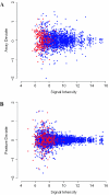
Figure 1

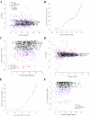
(A) Distribution of array deviates as a function of signal intensity. Red dots are the genes with only two successful arrays; blue dots are genes with three successful arrays. The magnitude of the errors depends on signal intensity, with larger errors at low-signal intensity, and smaller errors at high-signal intensity. Thus the distribution of errors is not log–normal, and so the error model requires an approach that includes dependence of error on signal intensity. The magnitude of the array deviates does not appear to depend on the number of successful arrays. (B) Similar plot for the feature deviates. The plot shows very similar behaviour, with a dependence of error on signal intensity. The magnitude of the feature deviates is slightly smaller than the array deviates.

Figure 2

(A) MVA plot for the array for infection with the EPEC strain after 6 h. Each gene is represented by one spot, which is colour coded according to the FDR associated with its P-value. The fold ratio at which genes are called differentially expressed depends on its signal intensity—with genes at higher signal intensity being differentially expressed at lower log ratios than genes at low-signal intensity. This is a reflection of the intensity-dependent error model. On the same axes we have plotted the standard deviation of the intensity-dependent error model distributions. There are three distributions: one for genes with one successful feature; one for genes with two successful features and one for genes with all three successful features. The distributions are most different at low-signal intensities, where the feature deviates are similar in magnitude to the array deviates. This is also the range of intensity where features are likely to fail. At high-signal intensities, where the magnitude of the feature deviates is much less than the magnitude of the array deviates, the distributions are dominated by the array deviates, and are very similar. In reality, features are much less likely to fail at high-intensity levels, so there is only a real need for the distribution for three successful replicates. (B) FDR plot for the EPEC strain array. On the x-axis we plot the P-value of the genes on a log (base 10) scale; on the y-axis we plot the FDR associated with that gene. This is essentially the expected number of false positives (equal to the number of genes in the analysis multiplied by the P-value), divided by the observed number of genes with P-values less than or equal to the P-value (i.e. the rank of the gene with this P-value). On this array, there are 804 genes in the analysis. We use the FDR curve to select differentially expressed genes. There are 27 genes with FDR <5% and 36 genes with FDR <10%. (C) Plot of average signal intensity against P-value for the genes in the EPEC ΔlifA mutant array. This is a diagnostic plot to determine the performance of our error model. Each spot represents a gene, and has been colour-coded according to the FDR associated with its P-value. There is no dependence of P-value on signal intensity, suggesting that our error model is performing well with these data. Furthermore, the FDR thresholds also do not depend on signal intensity, again supporting the use of our error model with these data. This contrasts with the MVA plot of log ratio against signal intensity, where there are more extreme log ratios at lower signal intensities than at higher signal intensities. The use of fold-ratio thresholds, or any other approach that does not include dependence of error on signal intensity, would be inappropriate with these data. (D) MVA plot of log ratio against signal intensity for the array for the EPEC ΔlifA mutant after 6 h. The results on this array show a far greater dependence of log ratio on signal intensity, with many more extreme values at low intensity, and fewer extreme values at high intensity. As with the ΔlifA, the analysis selects differentially expressed genes at high-signal intensities with lower fold ratios than the differentially expressed genes at low-signal intensities. (E) FDR plot for the ΔlifA mutant array. The FDR shows a similar behaviour. The top 29 genes have FDR <5% and the top 35 genes have FDR <10%. (F) Diagnostic plot of P-value against signal intensity for the ΔlifA mutant array. In general, there is no dependence of P-value on signal intensity. Similarly, there is no dependence of the FDR on signal intensity. However, there are two genes (BCL-2 antagonist of cell death and RAR-e) in the bottom-left-hand corner of the plot with very low-signal intensity and P-values. From this plot, we would suspect that these genes are outliers and do not represent truly differentially expressed genes. Furthermore, both these genes have only one successful feature, indicating that these data are likely to be less reliable.

Figure 3

Choice of the window width. The figure shows the percentage of genes detected (ordinate) as significant at given FDR as a function of window width (abscissa). It can be noted that the percentage of genes detected stabilizes around D = 150 independently of the FDR threshold.

Figure 4

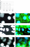
Characterization of EPEC and EHEC infection. (A) The percentage of Caco-2 cells infected with EPEC O127:H6 (EPEC), EHEC O157:H7 Sakai (stx^−/−) (EHEC), EPEC O127:H6 ΔlifA (EPEC dlifA) and EHEC O157:H7 Sakai (stx^−/−) Δler (EHEC dler) is shown. The graph clearly shows that the majority of cells are infected in all strains tested except the EHEC Δler. (B–G) The result of immunofluorescence assay is shown. The images of Caco-2 cell infected with EPEC O127:H6 and EHEC O157:H7 Sakai (stx^−/−) for 2 h are represented respectively in (F) and (G), and (D) and (E). Control Caco-2 cells (non-infected) are shown in (B and C). In (B, D and F), only the DAPI fluorescence is shown, whereas in (C, E and G) the merged fluorescence of both phalloidin (staining the cytoskeleton) and DAPI is shown. Red dashed circles in (D and F) indicate the position of the bacteria. In control cells actin microfilaments are diffused through the entire cell, while in infected cells they are clustered underneath the bacteria. It is noticeable that the morphology of the remodelling induced by EPEC O127:H6 and EHEC O157:H7 Sakai (stx^−/−) was different.

Figure 5

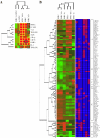
Cluster analysis. (A and B) The results of a two-way hierarchical clustering are shown. Samples are: Caco-2 cells infected for 6 h with EPEC O127:H6 (EPEC), EPEC O127:H6 ΔlifA (EPEC dlifA), EHEC O157:H7 Sakai (stx^−/−) (EHEC), EHEC O157:H7 Sakai (stx^−/−) Δler (EHEC dler) and EHEC O157:H7 Sakai (stx^−/−) (EHEC fix) and EPEC O127:H6 (EPEC fix) fixed; versus uninfected control Caco-2 cells. (A) The results of clustering using a subset of genes known to be downstream to NF-κB activation are shown. Highly significant ratios (FDR ≤10%) are marked in the heat map by yellow boxes. Significant genes (FDR >10% and <20%) are marked by black boxes. (B) The results of a two-way hierarchical clustering of genes that is differentially expressed (FDR ≤10%) in at least one of the arrays are shown. Dendrograms and heat maps are flanked by a colour-coded map representing genes associated with an FDR above (blue) and below (red) the chosen threshold in each array.

Figure 6

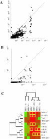
Comparison with the Rocke–Lorenzato two-component error model. (A) Scatterplot comparing the P-values obtained with the Bootstrap error model (abscissa) with the P-values obtained with the Rocke–Lorenzato error model (ordinate) is displayed. (B) Scatterplot comparing the FDR obtained with the Bootstrap error model (abscissa) with the FDR obtained with the Rocke–Lorenzato error model (ordinate) is displayed. (C) The result of clustering using a subset of genes known to be downstream to NF-κB activation is shown. Ratios that are highly significant according to the Rocke–Lorenzato model (FDR ≤10%) are marked in the heat map by yellow boxes. The map is directly compared with Figure 5A, which shows the results of the analysis on NF-κB downstream genes with the Bootstrap error model.

References

1. Schena M., Shalon D., Davis R.W., Brown P.O. Quantitative monitoring of gene expression patterns with a complementary DNA microarray. Science. 1995;270:467–470. - PubMed
1. Chin K.V., Kong A.N. Application of DNA microarrays in pharmacogenomics and toxicogenomics. Pharm. Res. 2002;19:1773–1778. - PubMed
1. Butte A. The use and analysis of microarray data. Nature Rev. Drug. Discov. 2002;1:951–960. - PubMed
1. Heller M.J. DNA microarray technology: devices, systems, and applications. Annu. Rev. Biomed. Eng. 2002;4:129–153. - PubMed
1. Shirota Y., Kaneko S., Honda M., Kawai H.F., Kobayashi K. Identification of differentially expressed genes in hepatocellular carcinoma with cDNA microarrays. Hepatology. 2001;33:832–840. - PubMed
Publication types