An efficient Monte Carlo method for estimating Ne from temporally spaced samples using a coalescent-based likelihood

Abstract

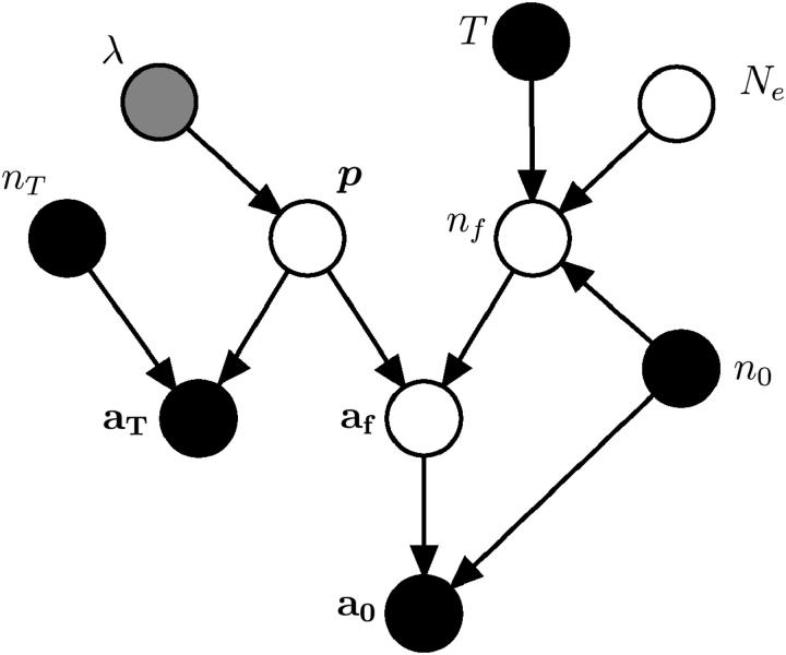
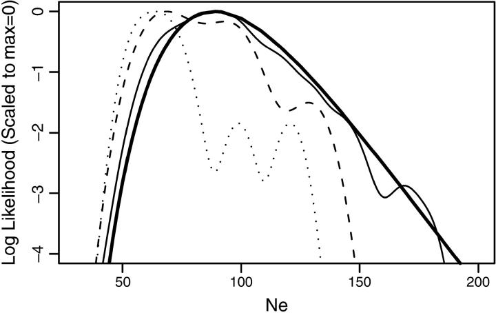
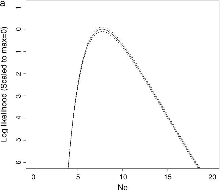
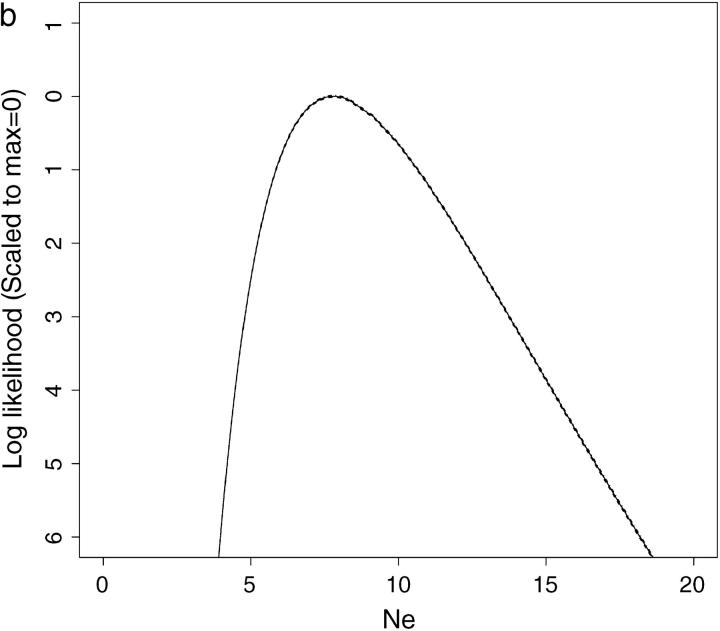
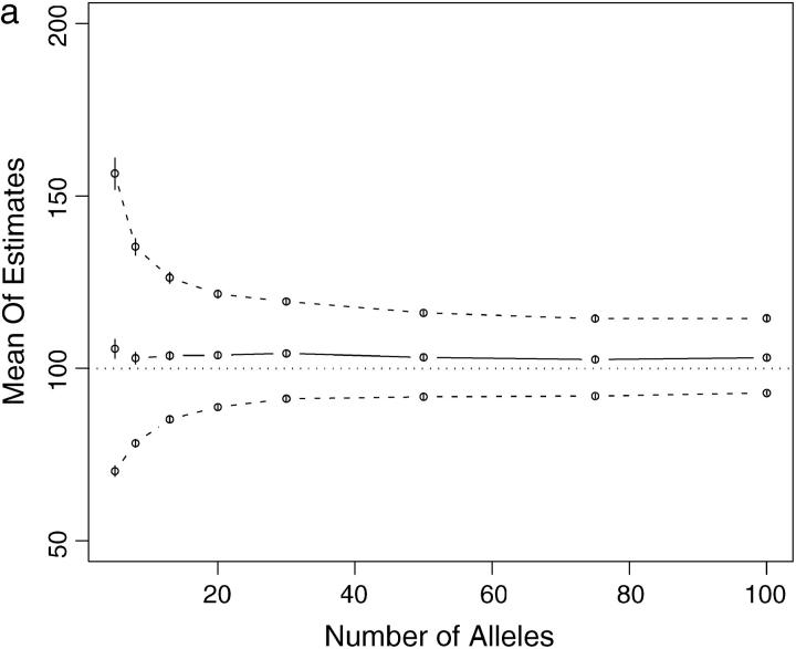
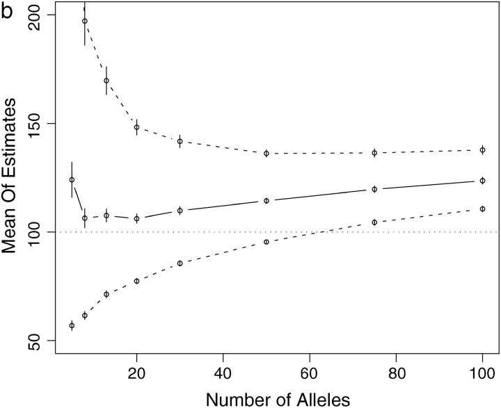
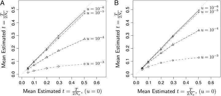
This article presents an efficient importance-sampling method for computing the likelihood of the effective size of a population under the coalescent model of Berthier et al. Previous computational approaches, using Markov chain Monte Carlo, required many minutes to several hours to analyze small data sets. The approach presented here is orders of magnitude faster and can provide an approximation to the likelihood curve, even for large data sets, in a matter of seconds. Additionally, confidence intervals on the estimated likelihood curve provide a useful estimate of the Monte Carlo error. Simulations show the importance sampling to be stable across a wide range of scenarios and show that the N(e) estimator itself performs well. Further simulations show that the 95% confidence intervals around the N(e) estimate are accurate. User-friendly software implementing the algorithm for Mac, Windows, and Unix/Linux is available for download. Applications of this computational framework to other problems are discussed.

Figure 1.—

A directed graph showing the relationship of the observed and latent variables in the probability model arising from the genealogical perspective. Each node represents a variable in the model. Solid nodes represent observed quantities, the shaded node represents a variable whose value is assumed to provide a prior distribution, and open nodes represent unobserved variables or, in the case of N_e, the unknown parameter of interest.

Figure 2.—

Comparison of estimated log L(N_e) between CoNe and TM3. The thick solid line shows the estimated log-likelihood curve produced by CoNe in 2 sec. Results from runs of TM3 that required 20, 200, and 2000 sec are shown by the dotted, dashed, and light solid line, respectively.

Figure 3.—

The worst Monte Carlo error from 30,000 data sets. (a and b) Solid lines are the estimated likelihood curves and dashed lines are the 95% confidence intervals around the estimated likelihood curves. The data set analyzed here had the widest confidence intervals of all 30,000 data sets analyzed for Table 1. It had 20 loci with five alleles. (a) Results for a CoNe run with m = 1000 Monte Carlo replicates, requiring <6 sec on a 2-GHz G5 processor. (b) Results for m = 50,000 Monte Carlo replicates, requiring 4 min 3 sec on the same processor. The dashed lines are difficult to see in b since the confidence interval around the likelihood curve is very narrow. Clearly the Monte Carlo error is minimal, and it is easily reduced by using more Monte Carlo replicates.

Figure 3.—

The worst Monte Carlo error from 30,000 data sets. (a and b) Solid lines are the estimated likelihood curves and dashed lines are the 95% confidence intervals around the estimated likelihood curves. The data set analyzed here had the widest confidence intervals of all 30,000 data sets analyzed for Table 1. It had 20 loci with five alleles. (a) Results for a CoNe run with m = 1000 Monte Carlo replicates, requiring <6 sec on a 2-GHz G5 processor. (b) Results for m = 50,000 Monte Carlo replicates, requiring 4 min 3 sec on the same processor. The dashed lines are difficult to see in b since the confidence interval around the likelihood curve is very narrow. Clearly the Monte Carlo error is minimal, and it is easily reduced by using more Monte Carlo replicates.

Figure 4.—

Summary of simulations using loci with different numbers of alleles. Points on solid lines show mean maximum-likelihood estimates from 250 simulated data sets as a function of number of alleles. See text for full explanation of simulations. Points on dashed lines show mean of upper and lower 95% confidence intervals for N_e. Vertical bars are two times the standard error of the mean in all cases. The thin dotted line shows the true value of N_e = 100. (a) Scaled time = 0.1, corresponding to 20 generations of drift with N_e = 100. (b) Scaled time = 0.01, corresponding to 2 generations of drift with N_e = 100. Note the upward bias in b.

Figure 4.—

Summary of simulations using loci with different numbers of alleles. Points on solid lines show mean maximum-likelihood estimates from 250 simulated data sets as a function of number of alleles. See text for full explanation of simulations. Points on dashed lines show mean of upper and lower 95% confidence intervals for N_e. Vertical bars are two times the standard error of the mean in all cases. The thin dotted line shows the true value of N_e = 100. (a) Scaled time = 0.1, corresponding to 20 generations of drift with N_e = 100. (b) Scaled time = 0.01, corresponding to 2 generations of drift with N_e = 100. Note the upward bias in b.

Figure 5.—

The effect of mutation on estimates of t = T/(2N_e) under the infinite-alleles model (A) and the K-allele model (B). In A and B the x-axis plots the mean from 300 simulated data sets of the estimate of t, when the true value of t was 0.05, 0.1, 0.2, 0.3, or 0.5 and the mutation rate is zero. The y-axis shows the mean estimated t from 300 data sets simulated with mutation at a rate u as indicated by the text to the right of each line. If mutation is causing no bias in the estimate, then the points will fall along the y = x line, which is indicated by the dotted line. Higher values of the mutation rate and higher values of the true t between sampling episodes increase the amount of bias that mutation causes. A downward bias in the estimate of t means an upward bias in the estimate of N_e.

References

1. Anderson, E. C., E. G. Williamson and E. A. Thompson, 2000. Monte Carlo evaluation of the likelihood for Ne from temporally spaced samples. Genetics 156: 2109–2118. - PMC - PubMed
1. Baum, L. E., 1971. Statistical inference for probabilistic functions of finite state Markov chains. Ann. Math. Stat. 37: 1554–1563.
1. Beaumont, M. A., 2003. Estimation of population growth or decline in genetically monitored populations. Genetics 164: 1139–1160. - PMC - PubMed
1. Beerli, P., and J. Felsenstein, 1999. Maximum-likelihood estimation of migration rates and effective population numbers in two populations using a coalescent approach. Genetics 152: 763–773. - PMC - PubMed
1. Berthier, P., M. A. Beaumont, J. M. Cornuet and G. Luikart, 2002. Likelihood-based estimation of the effective population size using temporal changes in allele frequencies: a genealogical approach. Genetics 160: 741–751. - PMC - PubMed
Publication types