Sedimentation velocity analysis of heterogeneous protein-protein interactions: sedimentation coefficient distributions c(s) and asymptotic boundary profiles from Gilbert-Jenkins theory

Abstract

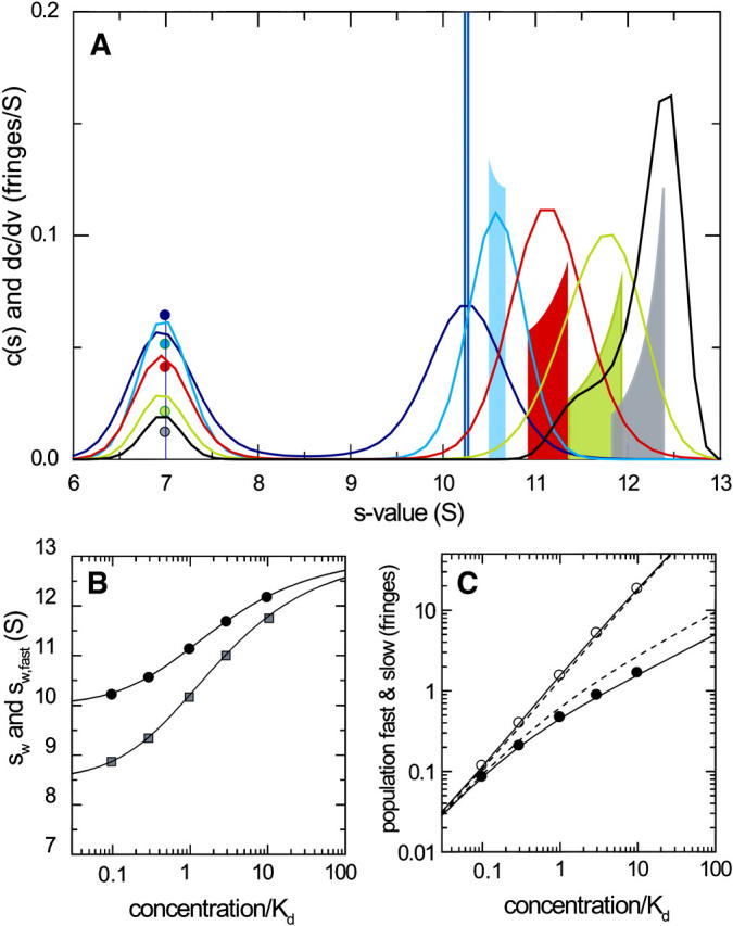
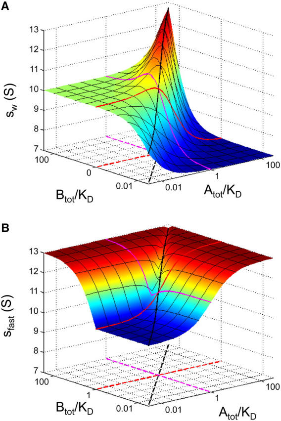
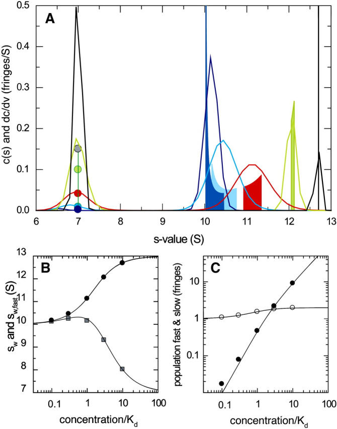
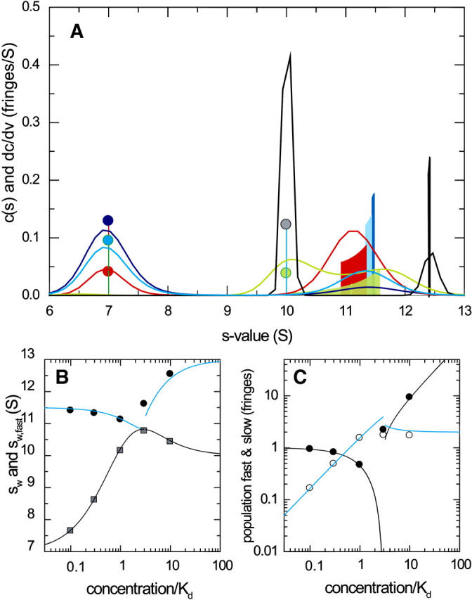
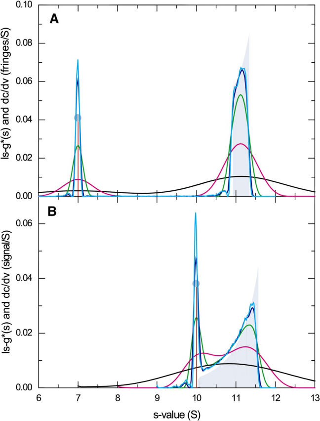
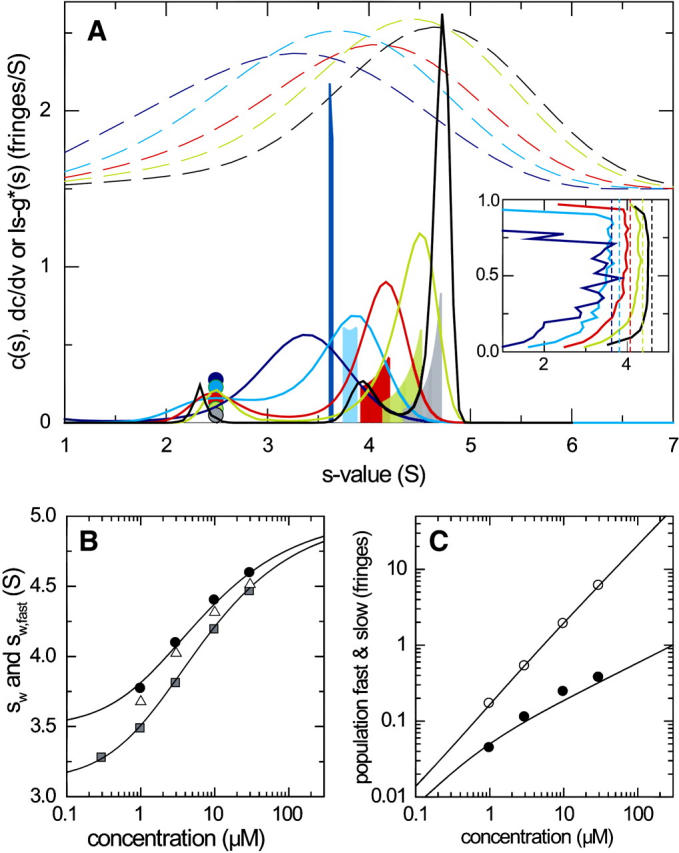
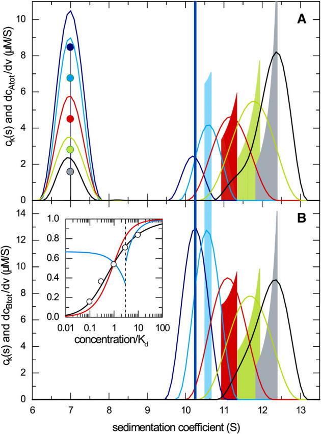
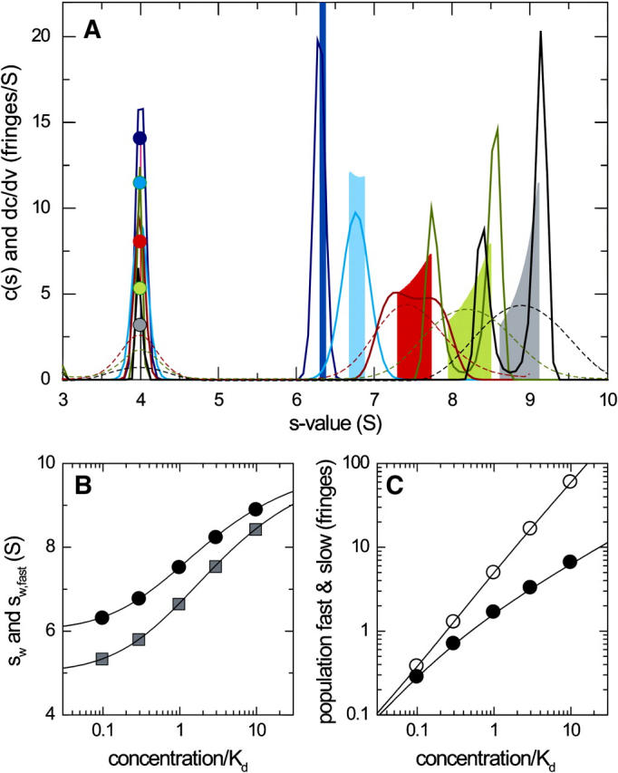
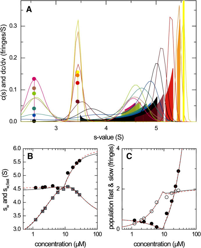
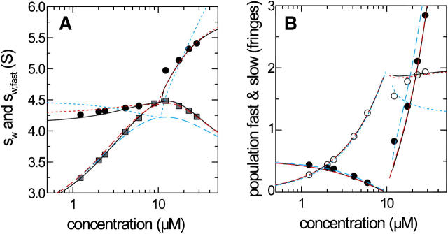
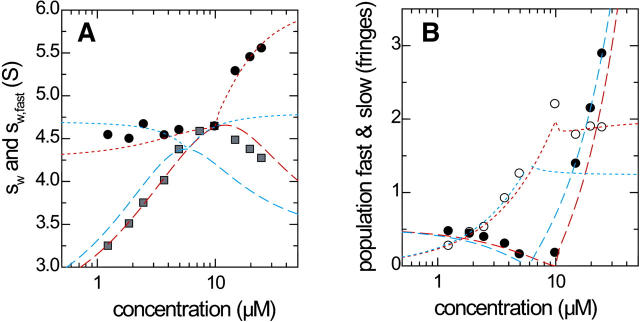
Interacting proteins in rapid association equilibrium exhibit coupled migration under the influence of an external force. In sedimentation, two-component systems can exhibit bimodal boundaries, consisting of the undisturbed sedimentation of a fraction of the population of one component, and the coupled sedimentation of a mixture of both free and complex species in the reaction boundary. For the theoretical limit of diffusion-free sedimentation after infinite time, the shapes of the reaction boundaries and the sedimentation velocity gradients have been predicted by Gilbert and Jenkins. We compare these asymptotic gradients with sedimentation coefficient distributions, c(s), extracted from experimental sedimentation profiles by direct modeling with superpositions of Lamm equation solutions. The overall shapes are qualitatively consistent and the amplitudes and weight-average s-values of the different boundary components are quantitatively in good agreement. We propose that the concentration dependence of the area and weight-average s-value of the c(s) peaks can be modeled by isotherms based on Gilbert-Jenkins theory, providing a robust approach to exploit the bimodal structure of the reaction boundary for the analysis of experimental data. This can significantly improve the estimates for the determination of binding constants and hydrodynamic parameters of the complexes.

FIGURE 1

Sedimentation boundary analysis of a reacting system A + B ↔ AB at a series of equimolar total concentrations. Theoretical sedimentation data were calculated by solving the Lamm equation for a 100-kDa, 7-S component A, and a 200-kDa, 10-S component B forming a 13-S complex in instantaneous local equilibrium, with 0.005 fringes normally distributed noise added. (A) Sedimentation coefficient distributions c(s) from the best-fit model of the simulated sedimentation data (solid lines) are shown at concentrations of 0.1-fold K_D (dark blue), 0.3-fold K_D (light blue), K_D (red), threefold K_D (green), and 10-fold K_D (gray), in units of fringes/S. The shapes of the asymptotic reaction boundaries dc/dv calculated for the same parameters are shown as solid bars, with the corresponding infinitely sharp undisturbed boundary indicated as solid circles (shown in fringe units). For clarity, both the c(s) and the dc/dv distributions were normalized to the same loading concentrations, and the reaction boundary of dc/dv was reduced fivefold in scale. (B) Isotherms of the signal-average s-value of the reaction boundary, s_fast, as derived from integration of the fast c(s) peak only (black circles), and s_w of the total sedimenting system derived from integration of the complete c(s) distribution (gray squares). The solid lines are the theoretically expected isotherms from GJT (Eq. 4) and the composition following mass action law for the system at rest (Eq. 5), respectively. (C) Signal amplitudes c_fast (○) and c_slow (•) of the two boundary components determined by integration of the c(s) peaks, and corresponding isotherms determined by GJT (solid lines). The short-dashed lines indicate the isotherms for the population of free A and (free B+AB) calculated by mass action law.

FIGURE 2

Isotherms of the theoretical concentration dependence of the weight-average sedimentation coefficient, s_w (A), and of the reaction boundary, s_fast (B). Sedimentation and interaction parameters are the same as those in Fig. 1. s_w(c_A,tot,c_B,tot) was calculated on the basis of the mass action law for the composition of the system at rest (Eq. 5), and s_fast(c_A,tot,c_B,tot) was calculated from GJT (Eq. 4). The lines indicate the configurations used to explore the sedimentation behavior of this system. They correspond to one-dimensional isotherms for the equimolar dilution series shown in Fig. 1 (black lines), the titration of a constant concentration of larger species with variable concentrations of the smaller species shown in Fig. 3 (red lines), and the titration of a constant concentration of the smaller species with variable concentrations of the larger species shown in Fig. 4 (magenta lines). Any experimental configuration of data points sampling the shape of the isotherms will be sufficient for the estimation of s_AB and K_D.

FIGURE 3

Sedimentation boundary analysis of a reacting system A + B ↔ AB at a constant concentration of the larger species B, in a titration series with the smaller species A. Sedimentation parameters were the same as those in Fig. 1, with sedimentation coefficients of 7 S and 10 S for the species A and B, respectively, forming a 13-S complex. (A) Sedimentation coefficient distributions c(s) from the best-fit model of the simulated sedimentation data (solid lines) are shown at concentrations of 0.1-fold K_D (dark blue), 0.3-fold K_D (light blue), K_D (red), threefold K_D (green), and 10-fold K_D (gray), in units of fringes/S. The presentation is analogous to Fig. 1. (B) Isotherms of s_fast as derived from integration of the fast c(s) peak (black circles), and s_w from integration of the complete c(s) distribution (gray squares). The solid lines are the theoretically expected isotherms for s_fast from GJT (Eq. 4) and for s_w from mass action law at rest (Eq. 5), respectively. (C) Signal amplitudes c_fast (○) and c_slow (•) as determined by integration of the c(s) peaks, and corresponding isotherms determined by GJT (solid lines).

FIGURE 4

Sedimentation boundary analysis of a reacting system A + B ↔ AB at a constant concentration of the smaller species A (7 S), in a titration series with the larger species B (10 S). Sedimentation parameters and labels are the same as those described in Fig. 3. For clarity, the isotherms of s_fast and c_fast are shown in blue in panels B and C.

FIGURE 5

A comparison of the boundary shapes predicted by GJT for rectangular cells at infinite time with Lamm equation solutions of sedimenting, reacting particles in the limit of very small diffusion coefficients. Lamm equations were solved for the same parameters as shown in Figs. 1 and 4, respectively, with the diffusion coefficient reduced by a factor 10⁴ (cyan), 10³ (blue), 100 (green), 10 (magenta), and unreduced (black), using the algorithm for a semiinfinite solution column (26). The simulated sedimentation profiles were transformed into sedimentation coefficient distributions using the ls − g*(s) method (50). For comparison, the profiles dc/dv are shown as gray bars and circles for the reaction and undisturbed boundary, respectively. The profiles were normalized to the same area. (A) Simulation under the same conditions as in Fig. 1, with equimolar loading concentration of A and B equal to K_D. (B) The same conditions as in Fig. 4 with a threefold molar excess of B over A.

FIGURE 6

Comparison of c(s) and the asymptotic boundary shape dc/dv for small species. Sedimentation conditions were analogous to those shown in Fig. 1, but simulating the interaction of a protein of 25-kDa, 2.5-S binding to a 40-kDa, 3.5-S species forming a 5-S complex with a equilibrium dissociation constant K_D = 3 μM, and a dissociation rate constant k_off = 0.01/s, studied at 50,000 rpm. Interference optical detection was assumed, with noise level of 0.005 fringes. Concentrations were equimolar at 0.1-fold K_D (dark blue), 0.3-fold K_D (light blue), K_D (red), threefold K_D (green), and 10-fold K_D (gray). The presentation of the results is as indicated in Fig. 1. The dashed lines in panel A are g*(s) distributions obtained from ls − g*(s) analysis of the simulated sedimentation profiles. The inset in panel A shows the integral sedimentation coefficient distributions G(s) from van Holde-Weischet analysis (41) (solid lines), and the expected s_fast (short-dashed vertical lines). Panel B presents the isotherms of s_fast (solid circles) and s_w (shaded squares) from c(s) and the theoretical expectation (solid lines). Also included for comparison are the maximum s-values of the G(s) distribution from van Holde-Weischet analysis (open triangles). Panel C presents the signal amplitudes c_fast (○) and c_slow (•) of the boundary components, respectively.

FIGURE 7

Multicomponent c_k(s) analysis compared with the components of the asymptotic reaction boundary dm_A,tot/dv and dm_B,tot/dv predicted by GJT. Sedimentation parameters were the same as those given in Fig. 1, and Lamm equation solutions were calculated simulating two signals, each with twofold different extinction coefficients for component A and B, respectively. Loading concentrations were equimolar at 0.1-fold K_D (dark blue), 0.3-fold K_D (light blue), K_D (red), threefold K_D (green), and 10-fold K_D (gray). The presentation is analogous to that of Fig. 1, with the scaled c_k(s) distributions obtained for component A in panel A, and the c_k(s) distribution obtained for component B in panel B. The inset in panel B shows the molar ratio of the components A/B as calculated from integrating the reaction boundary peak of the respective c_k(s) distributions (circles), and the theoretically expected molar ratio of the reaction boundary from GJT (black line). For comparison, the theoretical isotherm of the molar ratio in the reaction boundary for the titration of constant concentration of B with increasing concentrations of A (analogous to that of Fig. 3) is shown in red, and the reverse titration of constant A with increasing B (analogous to that of Fig. 4) is shown in blue.

FIGURE 8

Comparison of c(s) and dc/dv for the sedimentation of a two-site reaction A + 2B ↔ AB + B ↔ ABB with equivalent noncooperative sites. Sedimentation profiles were calculated on the basis of Lamm equation solutions with explicit reaction terms for instantaneous local equilibrium. The parameters were based on a molecule A (100 kDa, 6 S) with two identical noncooperative sites available for binding of a smaller ligand molecule B (50 kDa, 4 S), resulting in 8-S and 10-S complexes. Simulated concentrations were for A: 0.1-fold K_D,1 (dark blue), 0.3-fold K_D,1 (light blue), K_D,1 (red), threefold K_D,1 (green), and 10-fold K_D,1 (gray), and B in twofold molar excess of A, respectively. (A) Sedimentation coefficient distributions c(s) (solid lines, in units of fringes/S) for P = 0.9, and asymptotic reaction boundaries dc/dv calculated for the same parameters (solid bars, in units of fringes/S), with the corresponding undisturbed boundary indicated as solid circles (shown in fringe units). For comparison, the short-dashed lines indicate c(s) profiles calculated for the three highest concentrations with a frictional ratio fixed at 1.3. (B) Isotherms of s_fast, as derived from integration of the fast c(s) peak only (black circles), and s_w of the total sedimenting system derived from integration of the complete c(s) distribution (gray squares). The solid lines are the theoretically expected isotherms for s_fast from GJT (Eq. 4) and for s_w from mass action law at rest (Eq. 5), respectively. (C) Signal amplitudes c_fast (○) and c_slow (•) determined by integration of the c(s) peaks of the boundary components, and corresponding isotherms determined by GJT (solid lines).

FIGURE 9

Comparison of c(s) and dc/dv for the sedimentation of a two-site reaction A + 2B ↔ AB + B ↔ ABB for small molecules. Sedimentation profiles were calculated as Lamm equation solutions with explicit reaction terms. The parameters were based on a molecule A (31 kDa, 2.66 S) with two identical noncooperative sites for binding of a smaller ligand molecule B (45 kDa, 3.56 S), resulting in 4.96- and 6.11-S complexes. An instantaneous reaction was assumed. Simulated concentrations were at constant 4.96 μM for A, and 1.24 (magenta), 2.05 (light gray), 2.44 (light green), 4.20 (light blue), 6.04 (blue), 9.14 (black), 12.4 (violet), 17.7 (red), 23.3 (orange), 28.7 (yellow) μM for B, respectively, with equivalent noninteracting sites with the macroscopic binding constant of site one of K_D,1 = 1.7 μM. (A) Sedimentation coefficient distributions c(s) based on a fit with optimized meniscus position, optimized f/f₀, and with the regularization scaled to P = 0.9 (solid lines, normalized, in units of fringes/S), and asymptotic reaction boundaries dc/dv calculated for the same parameters (solid bars, in units of fringes/S), with the corresponding undisturbed boundary indicated as solid circles (shown in fringe units). (B) Isotherms of s_fast, as derived from integration of the fast c(s) peak (black circles), and s_w of the total sedimenting system derived from integration of the complete c(s) distribution (gray squares). The black solid lines are the theoretically expected isotherms for s_fast from GJT (Eq. 4) and for s_w from mass action law at rest (Eq. 5), respectively; the red short-dashed lines are the corresponding best-fit isotherms, resulting in s-values for the complexes of 5.23 and 6.20 S, respectively, and a binding constant K_D,1 of 2.4 μM. (C) Signal amplitudes c_fast (○) and c_slow (•) determined by integration of the c(s) peaks, and corresponding isotherms expected by GJT (solid lines) and from the best fit of GJT isotherms (red short-dashed lines).

FIGURE 10

The effect of finite reaction kinetics on the isotherm analysis. Sedimentation profiles were simulated using the Lamm equation solution for the same conditions as presented in Fig. 9, but with a finite reaction rate characterized by a chemical off-rate constant of 2.5 × 10⁻³/s. Panel A shows the isotherms of s_fast (circles) and s_w (squares), respectively, as determined from integration of c(s) of the simulated data (symbols), and predicted from GJT and initial composition (black lines). The red lines indicate the best-fit isotherms with a 2:1 model (short-dashed and long-dashed lines for s_fast and s_w, respectively), the blue lines the best-fit isotherms from an impostor single-site model. Panel B shows the signal amplitudes c_fast (○) and c_slow (•) determined by integration of the c(s) peaks, and corresponding isotherms expected by GJT (solid lines) and from best fit of GJT isotherms (red lines) and from an impostor single-site model (short-dashed and long-dashed lines for c_fast and c_slow, respectively).

FIGURE 11

Analysis of experimental data from the sedimentation of a natural killer cell receptor Ly49C (31 kDa) interacting with a MHC molecules H-2Kb (45 kDa) sedimenting at 50,000 rpm (35). The experimental parameters and best-fit sedimentation parameters from Lamm equation modeling (26) are equivalent to those simulated in Fig. 10. Panel A shows s_fast (circles) and s_w (squares), respectively, as determined from integration of c(s) (symbols). The red lines indicate the best-fit GJT isotherms with a 2:1 model, the blue lines the best-fit isotherms from an impostor single-site model.

References

1. Gilbert, G. A., and R. C. Jenkins. 1956. Boundary problems in the sedimentation and electrophoresis of complex systems in rapid reversible equilibrium. Nature. 177:853–854. - PubMed
1. Gilbert, G. A. 1959. Sedimentation and electrophoresis of interacting substances. I. Idealized boundary shape for a single substance aggregating reversibly. Proc. R. Soc. Lond. A. 250:377–388.
1. Gilbert, G. A., and R. C. Jenkins. 1959. Sedimentation and electrophoresis of interacting substances. II. Asymptotic boundary shape for two substances interacting reversibly. Proc R. Soc. Lond. A. 253:420–437.
1. Nichol, L. W., and A. G. Ogston. 1965. A generalized approach to the description of interacting boundaries in migrating systems. Proc. R. Soc. Lond. B Biol. Sci. 163:343–368.
1. Winzor, D. J., and H. A. Scheraga. 1963. Studies of chemically reacting systems on sephadex. I. Chromatographic demonstration of the Gilbert theory. Biochemistry. 2:1263–1267. - PubMed
LinkOut - more resources