Chevron behavior and isostable enthalpic barriers in protein folding: successes and limitations of simple Gō-like modeling

Abstract

It has been demonstrated that a "near-Levinthal" cooperative mechanism, whereby the common Gō interaction scheme is augmented by an extra favorability for the native state as a whole, can lead to apparent two-state folding/unfolding kinetics over a broad range of native stabilities in lattice models of proteins. Here such a mechanism is shown to be generalizable to a simplified continuum (off-lattice) Langevin dynamics model with a Calpha protein chain representation, with the resulting chevron plots exhibiting an extended quasilinear regime reminiscent of that of apparent two-state real proteins. Similarly high degrees of cooperativity are possible in Gō-like continuum models with rudimentary pairwise desolvation barriers as well. In these models, cooperativity increases with increasing desolvation barrier height, suggesting strongly that two-state-like folding/unfolding kinetics would be achievable when the pairwise desolvation barrier becomes sufficiently high. Besides cooperativity, another generic folding property of interest that has emerged from published experiments on several apparent two-state proteins is that their folding relaxation under constant native stability (isostability) conditions is essentially Arrhenius, entailing high intrinsic enthalpic folding barriers of approximately 17-30 kcal/mol. Based on a new analysis of published data on barnase, here we propose that a similar property should also apply to a certain class of non-two-state proteins that fold with chevron rollovers. However, several continuum Gō-like constructs considered here fail to predict any significant intrinsic enthalpic folding barrier under isostability conditions; thus the physical origin of such barriers in real proteins remains to be elucidated.

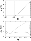
FIGURE 1

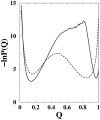
Enhancing cooperativity by imparting extra energetic favorability to the native state. (Upper panel) The solid curve shows the logarithmic density of states of a 27-mer Gō model in Kaya and Chan (26) with relative contact order CO = 224/756 = 0.296 and ground-state energy = −28; g(E) is number of conformations as a function of energy E estimated by standard Monte Carlo histogram techniques and sampling near the transition midpoint. The arrow and vertical lines mark the shift in ground state to E = −42 (E_gs = −14) for a thermodynamically more cooperative model as in Ref. 25. (Lower panel) Free energy profiles at the transition midpoints for the Gō (solid curve, ε/k_BT = −1.47) and the E_gs = −14 (dashed curve, ε/k_BT = −0.929) models, as the negative logarithm of their respective Boltzmann population P(Q), where Q is the fractional number of native contacts (note that P(Q = 27/28) = 0 for these models).

FIGURE 2

Comparing two native-centric models for the 64-residue truncated form of CI2 based on the native contact set NCS2, and the original and modified (scaled) “without-solvation” formulations at T = 0.82. Time in this and all subsequent figures is in units of simulation time step δt, as in Ref. 10. (a) A typical trajectory with many folding/unfolding cycles near the transition midpoint (ε = 0.81) of the original model, depicted by the time-dependence of Q (upper panel), and of kinetic energy (lower panel) given by where v_i values are the C_α velocities. (b) Corresponding data for a trajectory showing an unfolding/folding cycle near the transition midpoint (ε = 0.732) of the scaled model. Here the Q_ns = 117/142 level is marked by a horizontal line (upper panel). The example trajectory in b is from a continuous run: in this case, and unlike the procedure adopted for determining native population, Langevin dynamics of the scaled model was allowed to continue without interruption when the chain crosses over from Q < 117/142 to Q ≥ 117/142 (no restarting from a Q = 1 conformation at time ≈ 3.1 × 10⁸ for this particular trajectory). Key features of this continuous scaled-model trajectory are very much similar to that of trajectories simulated with Q = 1 restarts as described in the text (corresponding time-dependence data not shown).

FIGURE 3

The free energy profiles of the original Gō-like (dashed curve, ε/k_BT = 0.99) and the scaled (solid curve, ε/k_BT = 0.88) models in Fig. 2 are provided by the negative logarithm of their respective population P(Q) simulated at T = 0.82. Bias potentials and histogram techniques were employed to enhance sampling for the scaled model.

FIGURE 4

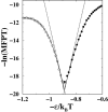
Chevron plot of the scaled CI2 model is given by the negative logarithmic mean first passage time (MFPT) of folding (open circles) and unfolding (solid circles) as functions of interaction strength −ε/k_BT. Results shown are for T = 0.82. The V-shaped lines constitute a hypothetical chevron plot consistent with the population-based free energy difference between the folded (Q ≥ 117/142) and unfolded (Q ≤ 25/142) conformations. MFPTs are averaged from 500 independent trajectories for −ε/k_BT ≤ −1.01 and −ε/k_BT ≥ −0.73, and 100 independent trajectories for −0.83 ≤ −ε/k_BT < −0.73, and −1.01 ≤ −ε/k_BT <−0.92. For the remaining −ε/k_BT values shown, each MFPT datapoint is averaged from ∼40 independent trajectories.

FIGURE 5

Isostability kinetic analysis of NTL9, an apparent two-state protein. (Left panel) Logarithmic folding rate (vertical axis, k_f in units of s⁻¹) versus native stability (free energy of folding in units of RT, horizontal axis) from varying denaturant concentration at constant temperature T₀ = 298.15 K (dotted straight line, ln k_f(ΔG_f/RT;T₀)) is compared with that from varying temperature T at zero denaturant (solid curve, ln k_f(ΔG_f/RT;T)). Thus, the native stability value at the point of intersection of the two sets of rates corresponds to that at T₀ and zero denaturant. This plot is based on the experimental measurement of Kuhlman et al. (4) of NTL9 in ²H₂O (pD 5.45) and using guanidine deuterium chloride (GuDCl) as denaturant. (Right panel) The difference between the two isostability logarithmic folding rates is essentially linear in 1/T, as stipulated by Eq. 11.

FIGURE 6

Isostability kinetic analysis reveals intrinsic Arrhenius relaxation in the folding of wild-type barnase. Data used in this analysis are from the experiments at pH 6.3 described in the text, using urea as denaturant. (Left panel) Logarithmic folding rate versus native stability from varying denaturant concentration at constant T₀ = 298.15 K (datapoints exhibiting less curvature along the dotted curve) is compared with that from varying T at zero denaturant (datapoints along solid curve). Notation and units are the same as that in Fig. 5. Here the dotted curve is a quadratic fit to the constant T = T₀ data, extrapolated to exhibit a hypothetical maximum folding rate at ΔG_f/RT ≈ −40 (24). (Right panel) The difference between the two isostability logarithmic folding rates of barnase (solid curve) is seen to vary essentially linearly with 1/T (compare to fitted dotted straight line).

FIGURE 7

A two-temperature isostability kinetic analysis of wild-type barnase in ²H₂O and guanidine hydrochloride (see text). (Left panel) Folding rate k_f (circles and squares) as a function of ΔG_f/RT for T₁ = 298.15K (25°C) and pD 7.5 are compared with that for T₂ = 310.15K (37°C) and pD 7.6. The fitted curves are guides for the eye. The k_f values are read off from the corresponding folding arms of the chevron plots in Fig. 1 of Ref. 46; the ΔG_f/RT values are obtained from the log K_N-D curves in Fig. 6 of the same reference by setting ΔG_f/RT = ln K_N-D. (Right panel) The approximate difference in logarithmic folding rate at the two temperatures as a function of ΔG_f/RT. This result is obtained directly from the fitted curves in the left panel. Here ln k_f(T₁) = ln k_f(ΔG_f/RT;T₁) and ln k_f(T₂) = ln k_f(ΔG_f/RT;T₂).

FIGURE 8

A lattice modeling scenario that assumes an intrinsic enthalpic barrier can reproduce trends from isostability kinetic analyses. Results in this figure are based on the model in Fig. 1 with ground-state energy = −42. (Left panel) Logarithmic folding rate versus native stability. The chain move set and all other aspects of the kinetic model are identical to that in Ref. 25; compare to Fig. 5 of this reference. ΔG_f is determined by standard Monte Carlo histogram techniques and sampling at ε/k_BT = −0.91. Here the dotted curve (with a smaller curvature) connects datapoints (not shown individually) of simulated constant-T logarithmic folding rates [ln k_f(ΔG_f/k_BT;T₀)], each averaged over 500 trajectories. This serves as a model for varying denaturant concentration. On the other hand, the solid curve provides the T-dependent logarithmic folding rate ln k_f(ΔG_f/k_BT;T), obtained by combining the dependence of ln k_f on the model zero-denaturant interaction strength ε₀/k_BT with a hypothetical T-dependence of ε₀ and a hypothetical T-dependent intrinsic conformational transition rate. Both hypothetical ingredients used here correspond to that in Fig. 7 b of Ref. 25. (Right panel) By construction, the difference between the two isostability logarithmic folding rates of this model is linear in 1/T.

FIGURE 9

The negative logarithmic folding (open symbols) and unfolding (solid symbols) MFPTs of the scaled model in Fig. 4 as functions of ε/k_BT at constant temperature (T = T₀ = 0.82, circles) are compared with corresponding logarithmic MFPTs simulated at different temperatures with a constant interaction energy parameter (ε = 0.725, squares). The V_stretching term in both sets of simulations are identical and independent of ε, with K_r = 72.5. The solid and dashed curves passing respectively through the circles and squares are guides for the eye. Definition of folding and unfolding first passage and the number of trajectories used in MFPT averaging are the same as that in Fig. 4.

FIGURE 10

Isostability kinetic analysis of the scaled model results in Fig. 9. (Left panel) Logarithmic folding rates are given by the negative logarithmic folding MFPTs in Fig. 9; ΔG_f is obtained by standard Monte Carlo histogram techniques (Figs. 3 and 4). Here ln k_f values from constant-T simulations (open circles, ln k_f(ΔG_f/k_BT;T₀)) and constant-ε simulations (solid circles, ln k_f(ΔG_f/k_BT;T)) are compared. (Right panel) The difference between the two model isostability logarithmic folding rates is essentially zero.

FIGURE 11

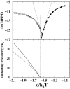
Isostability consideration of the without-solvation-SSR NCS2 model for CI2 in Kaya and Chan (10). (Upper panel) Negative logarithmic MFPTs for folding (open symbols) and unfolding (solid symbols) as functions of −ε/k_BT for variable-ε, constant temperature simulations (T = T₀ = 0.64, circles) and variable-T, constant ε simulations (ε = 0.99, squares); K_r = 99 for both sets of simulations. Each MFPT datapoint is averaged from ∼400 trajectories except ∼100 trajectories are used per datapoint around the transition midpoint. Fitted curves are guides for the eye. Folding simulations are initiated from a random conformation; first passage for folding is defined by the chain achieving Q = 1. Unfolding simulations are initiated from a Q = 1 conformation; first passage of unfolding is achieved when Q ≤ 25/142. (Lower panel) Native stabilities from histogram techniques are given here by the natural logarithm of the Boltzmann population of the folded state (Q ≥ 137/142) minus that of the denatured population with Q ≤ 35/142 (solid curve) and Q ≤ 80/142 (dashed curve). The V-shaped lines in the upper panel are a hypothetical two-state chevron plot consistent with the solid native stability curve in the lower panel. The vertical line indicates that there is a small mismatch between the thermodynamic and kinetic transition midpoints of this model. As in the original formulation of Kaya and Chan (10), the present Langevin formulation does not contain a δ-function-like force term for the apparent discontinuity in pairwise interaction at r_ij = 1.2 r′_ij as depicted in Fig. 3 b of Kaya and Chan for the without-solvation-SSR model. This implies that effectively all r_ij ≤ 1.2 r′_ij values of pairwise interaction energy for this model in Fig. 3 b of Kaya and Chan should be upshifted by −ε[5(1/1.2)¹² − 6(1/1.2)¹⁰] = 0.408ε such that the interaction energy is continuous. The conclusions of Kaya and Chan regarding the SSR models are not affected by this correction. Results from direct simulations (these include all kinetic data) remain unchanged. However, several results in Kaya and Chan that involve applications of thermodynamic histogram techniques need to be adjusted as follows: The heat capacity peaks of curves ii and iii in Fig. 5 of Kaya and Chan should be reduced to ≈3000 and 3500, respectively. The NCS2 stability curves and the hypothetical two-state chevron plot in Fig. 8 of Kaya and Chan should be replaced by the results in this figure; the corresponding corrections for NCS1 are very similar (data not shown). The front factor analysis for the without-solvation-SSR model in Fig. 12 d of Kaya and Chan should be replaced by the corresponding results in Fig. 13 b of the present article.

FIGURE 12

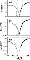
(a) Isostability consideration of the with-solvation NCS2 model for CI2 in Kaya and Chan (10), with the desolvation barrier height ε″ = 0.1ε. Notation and the kinetic definitions of folding and unfolding are identical to that for the upper panel of Fig. 11. Each MFPT datapoint here is averaged from ∼400 trajectories except ∼100 trajectories are used per datapoint around the transition midpoint. Fitted curves are mere guides for the eye. The variable-ε, constant temperature simulations (circles) are performed at T₀ = 0.82, whereas the variable-T, constant ε simulations (squares) are performed at ε = 0.92; K_r = 92 in both sets of simulations. The dashed V-shaped lines represent a hypothetical chevron plot that would be consistent with the population-based free energy difference between the folded and unfolded states determined from histogram techniques. The vertical double arrow marks a quasilinear (two-state-like) regime of the simulated chevron behavior. (b) Same as a except a higher pairwise desolvation barrier ε″ = 0.2ε is employed. Here ∼400 trajectories are used for each MFPT datapoint, except ∼50 trajectories each are used for MFPTs around the transition midpoint. (c) Same as a and b except for an even higher pairwise desolvation barrier ε″ = 5ε/9, and ε′ = ε/3. This prescription is identical to that of Cheung et al. (50). More than 150 trajectories are used to determine each of the MFPT datapoints shown. (Note that the expression (ε″ + ε′)/(ε′ − ε) on page 916 of Ref. 10 should read (ε″ + ε′)/(ε − ε′).) Owing to a technical oversight noted in the Corrigendum to Kaya and Chan (10), some results of the with-solvation models reported in Kaya and Chan were inaccurate. The errors are minor near the models' transition midpoint, as for Fig. 4 c and Fig. 6 of Kaya and Chan, but are larger under strongly folding and strongly unfolding conditions, necessitating the following corrections: The heat capacity curves iv and v in Fig. 5 of Kaya and Chan should both peak at k_BT ≈ 0.88 and each peak value should be reduced by ≈5%. The first passage time distribution in Fig. 11 c of Kaya and Chan and the estimated single-exponential slopes and t₀ should be replaced by the results in Fig. 13 of the present article. The front factor analysis for the with-solvation model in Fig. 12 d of Kaya and Chan should be replaced by the corresponding results in the present Fig. 13 b.

FIGURE 13

Single-exponential relaxation and front-factor contribution to chevron rollover. (a) Unfolding (open symbols) and folding (solid symbols) first passage time (FPT) distribution for the NCS2 with-solvation model in Fig. 12 a (circles). The corresponding NCS1 with-solvation model results (squares) are included for comparison (compare to Fig. 11 of Ref. 10). The vertical variable P(t)Δt is the probability for the FPT to lie within a range Δt around time t. The conditions for the present NCS1 unfolding and folding and NCS2 unfolding and folding are, in the same order, ε = 0.88, 0.98, 0.83, and 0.98; Δt/10⁵ = 5.0, 7.5, 2.0, and 1.5; and the number of trajectories simulated are 1500, 1200, 1500, and 1200, respectively. The corresponding set of least-square fitted {[10⁶ × (MFPT − t₀)⁻¹], [−10⁶ × slope]} values for self-consistency checks are {1.59, 1.72}, {0.99, 0.97}, {3.83, 4.32}, and {0.43, 0.44}. (b) Front factor analysis for folding (solid symbols) and unfolding (open symbols) of the present without-solvation-SSR model (squares) and with-solvation model in Fig. 12 a (circles). The vertical variable here is given by lnℱ = −ln(MFPT) + ΔG^‡/k_BT, where values of the kinetic activation quantity ΔG^‡/k_BT are defined as in Fig. 12 of Kaya and Chan (10) in terms of the order parameter Q along the free energy profiles of the models (detailed data not shown). Results in this figure are obtained using K_r = 100ε as in Ref. 10.

FIGURE 14

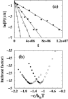
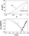
Thermodynamics and chevron behavior of the cooperative interaction scheme of Jewett et al. (30). The 27-mer lattice model in Fig. 1 is used in the present analysis. (Upper panel) The density of states of the common Gō model (solid curve, same as that in Fig. 1) is compared with that of the Jewett et al. interaction scheme (dashed curve). (Lower panel) Chevron plot of the Jewett et al. model. Folding (open circles) is initiated from a random conformation, and is completed when Q = 1. Besides the interaction scheme, the chain move set and other aspects of the kinetic model are identical to that in Kaya and Chan (25). Unfolding (solid circles) is initiated from the Q = 1 ground-state conformation, and unfolding first passage is achieved when Q ≤ 3/28. Each MFPT datapoint is averaged from 100 trajectories. The V-shaped lines is a hypothetical chevron plot consistent with the thermodynamic free energy difference between the folded (Q = 1) and unfolded (Q ≤ 3/28) conformations. Thermodynamic stability is estimated by standard Monte Carlo histogram techniques based on sampling at ε/k_BT = −1.35. The arrow marks the interaction strength at which ΔG_f = −10 k_BT.

FIGURE 15

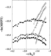
Chevron behavior of the 15-mer, three-dimensional, 20-letter lattice side-chain model of Klimov and Thirumalai (35). The interaction strength ε/k_BT here is equivalent to the parameter 1/T in the original reference. Folding simulations are initiated from the ground-state conformation (energy = −14.5). Unfolding simulations are initiated from randomly generated conformations. The solid squares, triangles, and circles are −ln(MFPT) values for folding with first passage defined respectively by energy becoming ≤−12.5, ≤−13.5, and ≤−14.5. The open squares, triangles, and circles are −ln(MFPT) values for unfolding with first passage defined respectively by energy reaching a value ≥−4.2, ≥−3.2, and ≥−2.2. Each simulated MFPT datapoint is averaged from 500 trajectories. Continuous lines and curves are mere guides for the eye. The move set used in the kinetic simulations consists of end, corner, crankshaft, and side-chain moves, as in the original reference. The vertical line marks the interaction strength at the heat capacity peak of this model (compare to Fig. 2 c of Ref. 35 and Fig. 9 of Ref. 71).

References

1. Jackson, S. E., and A. R. Fersht. 1991. Folding of chymotrypsin inhibitor 2. I. Evidence for a two-state transition. Biochemistry. 30:10428–10435. - PubMed
1. Chan, H. S., S. Shimizu, and H. Kaya. 2004. Cooperativity principles in protein folding. Methods Enzymol. 380:350–379. - PubMed
1. Scalley, M. L., and D. Baker. 1997. Protein folding kinetics exhibit an Arrhenius temperature dependence when corrected for the temperature dependence of protein stability. Proc. Natl. Acad. Sci. USA. 94:10636–10640. - PMC - PubMed
1. Kuhlman, B., D. L. Luisi, P. A. Evans, and D. P. Raleigh. 1998. Global analysis of the effects of temperature and denaturant on the folding and unfolding kinetics of the N-terminal domain of the protein L9. J. Mol. Biol. 284:1661–1670. - PubMed
1. Daggett, V. 2002. Molecular dynamics simulations of the protein unfolding/folding reaction. Acc. Chem. Res. 35:422–429. - PubMed
Publication types
Substances
LinkOut - more resources