Chromatic gain controls in visual cortical neurons

Abstract

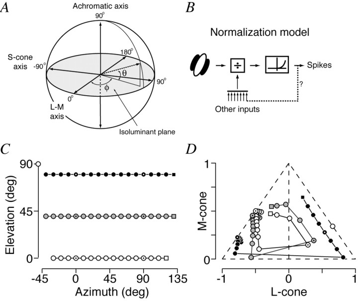
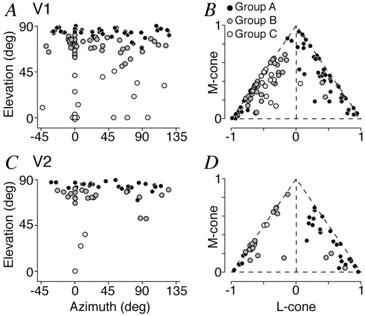
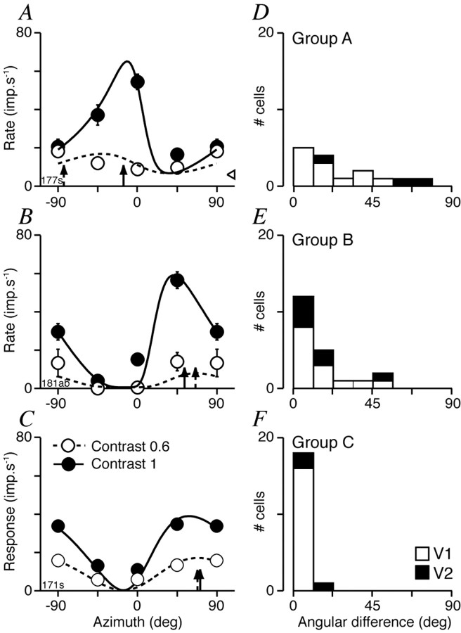
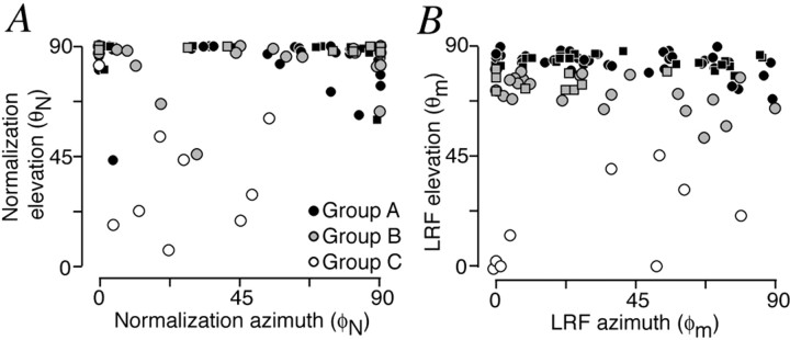
Although the response of a neuron in the visual cortex generally grows nonlinearly with contrast, the spatial tuning of the cell remains stable. This is thought to reflect the activity of a contrast gain control ("normalization") that has very broad tuning on the relevant stimulus dimension. Contrast invariant tuning on a particular dimension is probably necessary for reliable representation of stimuli on that dimension. In the lateral geniculate nucleus (LGN), V1, and V2 of anesthetized macaque, we measured chromatic tuning of neurons at several contrasts to characterize the gain controls and identify cells that might be important for representing color. We estimated separately the chromatic signature of the linear receptive field and that of the gain control. In the LGN, we found normalization in magnocellular cells and cells receiving excitatory S-cone input but not in parvocellular cells or those receiving inhibitory S-cone input. We found normalization in all types of cortical neurons. Among cells that preferred achromatic modulation, or modulation along intermediate directions in color space (making them responsive to both achromatic and chromatic stimuli), normalization was driven by mechanisms tuned to a restricted range of directions in color space, close to achromatic. As a result, chromatic tuning varied with contrast. Among the relatively few cells that strongly preferred chromatic modulation, normalization was driven by mechanisms sensitive to modulation along all directions in color space, especially isoluminant. As a result, chromatic tuning changed little with contrast. To the extent that contrast invariant tuning is important in representing chromaticity, relatively few cortical neurons are involved.

Figure 1.

A, Color space used to represent stimuli. It is defined by an L-M axis along which the signals of the L and M cones covary to keep their sum constant, an S-cone isolating axis, and an achromatic axis where the signals of the three cone classes vary in proportion. The L-M- and S-cone axes define an isoluminant plane, where chromaticity varies without a change in luminance. Stimuli are specified by their azimuth in the isoluminant plane (ϕ) and their elevation from the isoluminant plane (θ). B, Model cortical receptive field incorporating normalization pool [following Carandini et al. (1997)]. The LRF computes a weighted linear sum over local contrast and chromaticity. This signal is then divided by a normalization signal with a chromatic signature that can differ substantially from that of the receptive field. C, D, Relationship between the preferred azimuth and elevation of the LRF and the weights assigned to signals from different classes of cones. Each combination of azimuth and elevation represented by a point in C has a counterpart point in D that shows the weights on the three classes of cones. Each connected sets of points characterizes a different preferred elevation: 0° (open symbols), 40° (gray symbols), and 80° (filled symbols) at a range of azimuths. The isolated open symbol in D shows the cone weights associated with a preferred elevation of 90°. Symbols containing small dots represent LRFs with preferred azimuths of 0 and 90°. Conventions used in C: L- and M-cone inputs of the opposite sign are represented with negative L-cone weights; the strength of the S-cone input is represented by the distance inside the diagonal. In this and the following figures, degree is abbreviated as “deg.”

Figure 2.

Chromatic signatures of receptive fields in V1 and V2. A, C, Distributions of the preferred directions in the color space of Figure 1 A. B, D, Distributions of the relative weights attached to inputs from each cone class. Here and in subsequent figures, the different symbols distinguish the three groups of cells discussed in the text: group A, cells that preferred achromatic modulation (filled symbols); group B, cells that preferred modulation at intermediate elevations (gray symbols); group C, cells that preferred isoluminant modulation (open symbols). In A and C, the preferred azimuths and elevations have been reflected into a reduced space that does not distinguish cells with complementary signatures. In B and D, the true signs of cone inputs are unknown, so cells with L- and M-cone inputs of the opposite sign are shown with negative L-cone weights. The strength of S-cone input is represented by distance inside the diagonal.

Figure 3.

Three models of chromatic response regulation in a simple cell with a preferred elevation of 50° and a preferred azimuth of 0°. Each pair of panels shows response magnitude (top) and response phase (bottom) as a function of the wRMS contrast in the stimulus (see Materials and Methods for derivation). Responses are shown for three different directions of modulation in the L-M/achromatic plane: isoluminant (0° elevation), achromatic (90° elevation), and intermediate (45° elevation). A, Linear: response increases in proportion to contrast and phase is independent of contrast. B, Compressive nonlinearity: amplitude and phase depend only on the capacity of the stimulus to drive the receptive field. Amplitude asymptotes at the same level for all color directions, and phase begins to advance at different contrast levels. C, Normalization by a mechanism that is equally sensitive to modulation along all directions in color space: the shapes of contrast-amplitude and contrast-phase curves are determined in contrast, and not the effectiveness of a particular stimulus for the LRF. Response amplitudes asymptote at different values, and response phases are identical. The circles indicate the maximum contrast achievable along each color direction on our monitor. In this and the following figures, impulses is abbreviated as “imp.”

Figure 4.

Normalization in complex cells. A, Sets of contrast-response curves for a weakly opponent cell (group B) in V1. Top, Mean rate to stimuli modulated along the identified directions in the isoluminant plane (elevation, 0°). Middle, Mean rate to stimuli modulated along the identified elevations in the plane formed by the L-M axis (azimuth, 0°) and the achromatic axis. Bottom, Mean rate to stimuli modulated along the identified elevations in the plane formed by the S-cone axis (azimuth, 90°) and the achromatic axis. B, As for A, except for a weakly opponent (group B) complex cell in V2. Missing curves in the top and bottom panels reflect the absence of a response to modulation along the S-cone axis. Solid lines are the predictions of the normalization model described in Materials and Methods, fit to the mean response rates obtained. Model and stimulus parameters: for A, σ = 0.11, n = 3.9, θ_N = 88.1^o, ϕ_N = 9.0^o, 1.0 cycles · degree^-1, 5.3 Hz; for B, σ = 0.05, n = 4.6, θ_N = 88.4^o, ϕ_N = 0.0^o, 3.0 cycles · degree^-1, 4.8 Hz. Individual parameters estimated the height of each curve. Error bars are ±1 SEM from 20 repetitions. In this and the following figures, “Achrom” refers to the achromatic axis.

Figure 5.

Normalization in a simple cell. Sets of contrast-response curves for a weakly opponent cell (group B) in V1. A, Responses are shown for stimuli modulated along the identified elevations in the L-M/achromatic plane. The top and bottom panels show, respectively, response amplitude and phase at the frequency of modulation. The phase curves have been spaced vertically for clarity. B, Same as A, except the plane of modulation was S-cone/achromatic. Solid lines are the predictions of the normalization model described in Materials and Methods, fit to response amplitude and phase in the complex plane. Model and stimulus parameters: t₀ = 25.2 ms; t₁ = 6.7; n = 5.0; θ_N = 87.0^o; ϕ_N = 90.0^o; 1.4 cycles · degree^-1; 5.3 Hz. Individual parameters estimated the height of each curve. Error bars are ±1 SEM from 13 repetitions.

Figure 6.

Normalization in color-preferring cells (group C) in V1. A, Sets of contrast-response curves for a cell that preferred S-cone modulation. Responses are shown for stimuli modulated along the identified azimuths in the isoluminant plane (left) and the identified elevations in the plane formed by the S-cone and achromatic axes (right). The top and bottom panels show, respectively, response amplitude and phase at the frequency of modulation. B, Same as A, except for a cell that preferred L-M modulation; the right panels show responses to modulation in the L-M/achromatic plane. C, Same as A, for another cell that preferred S-cone modulation. Solid lines are the predictions of the normalization model described in Materials and Methods, fit to response amplitude and phase in the complex plane, for all color directions to which the cell responded (more than are shown). Model and stimulus parameters: for A, t₀ = 59.3 ms, t₁ = 15.4, n = 2.3, θ_N = 66.3^o, ϕ_N = 72.8^o, 0.5 cycles · degree^-1, 5.3 Hz; for B, t₀ = 29.3, t₁ = 9.0, n = 4.7, θ_N = 19.1^o, ϕ_N = 45.3^o, 0.0 cycles · degree^-1, 3.9 Hz; for C, t₀ = 10.1, t₁ = 3.2, n = 2.7, θ_N = 43.8^o, ϕ_N = 27.1^o, 0.5 cycles · degree^-1, 6.0 Hz. Individual parameters estimated the height of each curve. Error bars are ±1 SEM from 11 (A) or 20 (B, C) repetitions.

Figure 7.

Comparison of the predictive power of three models of response regulation. A, Comparison of unexplained variance from fits of the linear and normalization models for V1 neurons in our three groups. The variance left unexplained by each model was obtained from the response amplitude. B, Same as A, except for V2 neurons. C, Comparison of compressive and normalization models for V1 neurons. Other details are the same as for A. D, Same as C, except for V2 neurons. Points above the unit diagonal indicate that the normalization model provides a better overall description. The squares (A, C) and circles (B, D) plot the cells shown in Figures 4, 5, 6.

Figure 8.

Effect of contrast on chromatic tuning in the isoluminant plane. A, Responses of a V2 complex cell (group A) measured at moderate contrast and high contrast. B, C, Same as A, except for a V1 complex in group B and a V1 color-preferring cell in group C, respectively. Contrast has little effect on the preferred color direction for the group C cell, but for both group A and group B neurons, the change in contrast changed the preferred azimuth (notably so for the cell in A). Solid lines are the best-fitting predictions of the normalization model described in Results. D, Distributions of unsigned shifts in the preferred azimuth brought about by changing contrast from moderate to high in group A cells in V1 and V2. E, Same as D, except for group B cells. F, Same as D, except for group C cells. Model and stimulus parameters: for A, ϕ_M = -53.6^o, ϕ_N = 84.4^o, σ = 0.04, n = 2.3, 2.2 cycles · degree^-1, 5.3 Hz; for B, ϕ_M = 76.6^o, ϕ_N = 90.0^o, σ = 0.12, n = 5.0, 2.9 cycles · degree^-1, 3.9 Hz; for C, ϕ_M = 74.1^o, ϕ_N = 72.8^o, σ = 0.36, n = 2.3, 0.5 cyc.deg^-1, 5.3 Hz. Error bars are ±1 SEM from 15 (A), 7 (B), or 11 (C) repetitions.

Figure 9.

Chromatic signatures of normalization pools and LRFs. A, Distribution of preferred directions of normalization pools for cells in which they could be accurately determined (n = 103). Cell groups A-C are identified by the usual conventions; circles and squares identify, respectively, neurons in V1 and V2. B, Same as A, except for the LRFs of the same cells.

Figure 10.

Comparison of chromatic signatures of LRF and normalization pool. A, Preferred elevation of normalization pool versus preferred elevation of LRF for cells of Figure 9. Marginal histograms show the distributions of elevations for LRF (top) and the normalization pool (right). The white bars identify group C cells, and the black bars identify group A and B cells. B, Preferred azimuth of normalization pool versus preferred azimuth of LRF, for cells in A with preferred elevations of the normalization pool that differed significantly from the achromatic axis (n = 52). Marginal histograms show the distributions of azimuths for the LRF (top) and normalization pool (right). Conventions are the same as in A.

Figure 11.

Variation in normalization sensitivity with chromatic signature of the LRF. A, Normalization sensitivities of cells in the identified groups A-C in V1 (circles) and V2 (squares) versus the preferred elevation of the LRF. Normalization sensitivity was calculated from fits of the normalization model to the response amplitude. Histograms to the right show the distributions of normalization sensitivities for V1 and V2 cells (black, group A; gray, group B; white, group C). B, Normalization sensitivities for all cells in the LGN versus the preferred elevation of the LRF. The histogram to the right shows the distribution of normalization sensitivity (black, M-cells; gray, blue-ON cells; white, P-cells; white with black dot, blue-OFF cells).

Figure 12.

Normalization in P-cells and M-cells in the LGN. Sets of contrast-response curves for a P-cell (A) and an M-cell (B) are shown. Responses are shown for stimuli modulated along the identified elevations in the L-M/achromatic plane. Conventions are as in Figure 5. Model and stimulus parameters: for A, t₀ = 0.1 ms, t₁ = 11.1, n = 1.2, θ_N = 64.1^o, ϕ_N = 0.0^o, 0.0 cycles · degree^-1, 9.0 Hz; for B, t₀ = 65.6, t₁ = 7.5, n = 1.2, θ_N = 89.4^o, ϕ_N = 0.0^o, 1.0 cycles · degree^-1, 6.9 Hz. Error bars are ±1 SEM from 11 repetitions.

Figure 13.

Normalization in S-cone-driven cells in the LGN. Sets of contrast-response curves for a blue-ON cell (A) and a blue-OFF cell (B). Responses are shown for stimuli modulated along the identified elevations in the S-cone/achromatic plane. Conventions are as in Figure 5. Model and stimulus parameters: for A (dashed lines), t₀ = 6.6 ms, t₁ = 3.2, n = 1.2, θ_N = 20.8^o, ϕ_N = 90.0^o, 0.0 cycles · degree^-1, 5.0 Hz; for B, t₀ = 47.1, t₁ = 57.1, n = 1.3, θ _N = 0.0^o, ϕ_N = 0.0^o, 0.0 cycles · degree^-1, 5.0 Hz. Error bars are ±1 SEM from 11 repetitions.

Figure 14.

Chromatic signatures of neurons of different classes in the LGN. A, Distribution of preferred directions in the color space of Figure 1 A. B, Relative weights attached to inputs from each cone class. Conventions are as in Figure 2.

References

1. Abbott LF, Varela JA, Sen K, Nelson SB (1997) Synaptic depression and cortical gain control. Science 275: 220-224. - PubMed
1. Albrecht DG, Hamilton DB (1982) Striate cortex of monkey and cat: contrast response function. J Neurophysiol 48: 217-237. - PubMed
1. Benardete EA, Kaplan E (1997) The receptive field of the primate P retinal ganglion cell, II: nonlinear dynamics. Vis Neurosci 14: 187-205. - PubMed
1. Benardete EA, Kaplan E, Knight BW (1992) Contrast gain control in the primate retina: P cells are not X-like, some M cells are. Vis Neurosci 8: 483-486. - PubMed
1. Bonds AB (1989) Role of inhibition in the specification of orientation-selectivity of cells in the cat striate cortex. Vis Neurosci 2: 41-55. - PubMed
Publication types