Spatial invasion by a mutant pathogen

Abstract

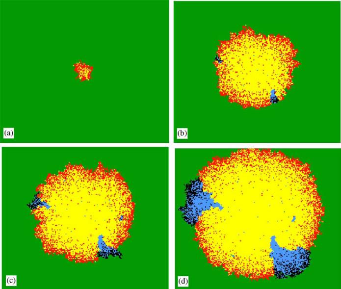
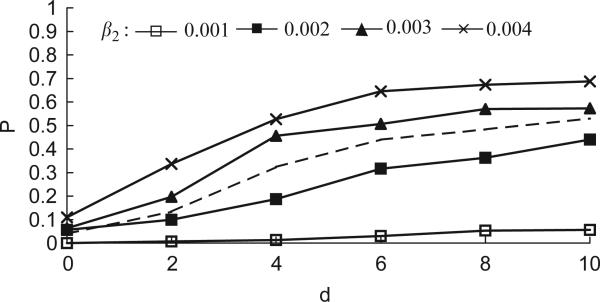
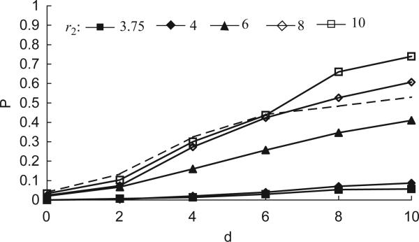
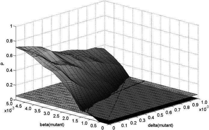
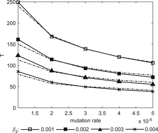
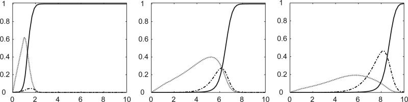
Imagine a pathogen that is spreading radially as a circular wave through a population of susceptible hosts. In the interior of this circular region, the infection dies out due to a subcritical density of susceptibles. If a mutant pathogen, having some advantage over wild-type pathogens, arises in this region it is likely to die out without leaving a noticeable trace. Mutants that arise closer to the infection wavefront have access to more susceptible hosts and thus are more likely to become established and perhaps (locally) out-compete the original pathogen. Among the factors (position, transmission rate, pathogen-induced death rate) that influence the fate of a mutant, which are most important? What does this tell us about the types of mutants that are likely to invade and become established? How do such tendencies serve to steer the evolution of pathogens in a spatial setting? Do different types of models of the same phenomena lead to similar conclusions? We address these issues from the point of view of an individual-based stochastic spatial model of host-pathogen interactions. We consider the probability of a successful invasion by a single mutant as a function of the transmissibility and virulence strengths and the mutant position in the wavefront. Next, for a version of the model in which mutations arise spontaneously, we obtain analytical and simulation results on the mean time to a successful invasion. We also use our model predictions to gain insight into experimental data on bacteriophage plaques. Finally, we compare our results to those based on ordinary and partial differential equations to better understand how different models might influence our predictions on the fate of a mutant pathogen.

Fig. 1

A typical simulation of the spontaneous mutation IPS model (green = susceptibles, red wild-type infectives, yellow = dead wild-type infectives, black = mutant infectives, blue = dead mutant infectives). (a) wild-type infection wave begins; (b) two mutant infective invasions getting started; (c) mutant infective colonies starting to emerge, with one unsuccessful invasion also evident; (d) clonal wedge pattern of two fully developed mutant pathogen colonies. Note that the “live” infectives are mostly on the edge. The clonal wedge pattern, evident only when we distinguish between different types of dead infectives, provides a historical perspective on the development of the spatial invasions. The parameter settings are β₁ = 0.002, δ₁ = 0.0002, β₂ = 0.0024, δ₂ = 0.00022, and μ = 0.0000001.

Fig. 2

Invasion probability as a function of mutant position d and transmission rate β₂, for a fixed ratio β₂/δ₂ = 10 that is significantly larger than the wild-type ratio. (Wild-type parameters β₁ = 0.002, δ₁ = 0.0005, β₁/δ₁ = 4 are held constant.) The dashed curve represents the success probability for a pathogen that has exactly the same transmission and mortality rates as the wild type. For β₂<β₁, the mutant pathogen has a difficult time, with invasion probability essentially tracking that of a neutral mutant until the distance from the wavefront is so large that there is not much chance for competition. When the mutant has the same transmission rate as the wild type, the effect of the larger ratio is seen to be significant. As we increase the mutant transmission rate past that of the wild type, the invasion probability increases somewhat but most of the gains are made at d = 0. This indicates the importance of transmission rate in determining whether the mutant is able to escape the initial congestion of the wavefront.

Fig. 3

Invasion probability as a function of mutant position d and transmission rate β₂, for a fixed ratio β₂/δ₂ = 3.75 that is smaller than the wild-type ratio (but still larger than the critical ratio). Other settings are as in Fig. 2.

Fig. 4

Invasion probability as a function of mutant position d and ratio r₂ = β₂/δ₂, for a fixed value of transmission rate β₂ = 0.001 that is smaller than that of the wild-type. Other settings are as in Fig. 2.

Fig. 5

Invadability threshold for a single mutant as a function of δ₂, β₂ (with δ₁ = 0.0002, β₁ = 0.002, β₁/δ₁ = 10 held constant). The dark triangles represent parameter values for which a fraction of at least 0.05 of the 300 runs resulted in a successful mutant invasion; the open circles correspond to invasion frequencies of less than 0.05. The dotted straight line gives the critical ratio r₂ = β₂/δ₂ = 3.5. The solid curve gives values of δ₂, β₂ satisfying the relation ${\beta }_2{r}_2^{1∕3}={\beta }_1{r}_1^{1∕3}$; dash-dot curve ${\beta }_2{r}_2^{1∕2}={\beta }_1{r}_1^{1∕2}$; dashed curve β₂r₂ = β₁r₁. The data indicate that for invasion to occur the parameters must correspond to points above both the critical ratio line and the solid curve, as specified in the invasion condition.

Fig. 6

Invasion probability surface corresponding to the parameters in Fig. 5. Also illustrated are the cutoff probability plane and the threshold curves. The straight line gives the critical ratio r₂ = 3.5 and the solid curve gives the parameters satisfying the relation ${\beta }_2{r}_2^{1∕3}={\beta }_1{r}_1^{1∕3}$.

Fig. 7

Dark curves show mean invasion time, $\stackrel{‒}{T}$, based on 300 runs as a function of mutation rate in the spontaneous mutation IPS model. The lighter companion curve for each of these gives the best fit of the form $E\left(T\right)=a∕\sqrt{\mu }$; cf. Eq. (4). The value of the constant a is simply chosen to overlay the two curves as much as possible so as to determine how well the dependence on mutation rate is matched. In all simulations, we fix the values β₁ = 0.002, r₁ = 4, and r₂ = 5.

Fig. 8

Comparison of values of ${(\stackrel{‒}{T^{\prime }}∕\stackrel{‒}{T})}^2$ (solid squares), based on spontaneous mutation simulations, and p/p′ (open squares), based on single mutant simulations; cf. Eq. (6). The numbers on the horizontal axis correspond to different parameter settings for the two mutant pathogens. If we write T1, T2, T3, T4 for the transmission rates 0.004, 0.003, 0.002, 0.001, then the six points on the horizontal axis correspond to the parameter settings $({\beta }_2,{\beta }_2^{\prime })$ of (T1, T2), (T1, T3), (T1, T4), (T2, T3), (T2, T4), (T3, T4). Held constant are r₁ = r₂ = 10, β₁ = 0.002, and δ₁ = 0.0002.

Fig. 9

Sampling regions along four equally spaced radii used to generate the invasion curves in Fig. 10. Each square contains 100 sites (10 × 10) and is intended to correspond to a “stab sample” in Yin's experiments. The colors in the simulation are as in Fig. 1.

Fig. 10

Invasion curves corresponding to the radial sampling regions in Fig. 9. Each row corresponds to one (completed) run of the simulation, with the four graphs in each row giving the fraction of mutant pathogens in sampling squares 1,2, etc., along each of the four different radii. The top two rows were obtained with parameter settings β₁ = 0.002, δ₁ = 0.00016, β₂ = 0.004, δ₂ = 0.00032, and μ = 10^–7; the bottom two rows were obtained with parameter settings β₁ = 0.002, δ₁ = 0.00016, β₂ = 0.0023, δ₂ = 0.00018, and μ = 10^–7. Note that larger values of β₂ lead to less variability in the invasion curves.

Fig. 11

Invasion in a traveling wave for RDE model. Parameters are β₁ = 0.002, δ₁ = 0.0005, β₂ = 0.0023, δ₂ = 0.0005, and D = 1. Solid curve gives susceptible density, dark dashed curve gives density of mutant infectives, and light dashed curve gives density of wild-type infectives. Three snapshots show the mutant arising at low density in the wavefront of the wild-type pathogen and then steadily taking over while the wild type dies out.

Fig. 12

Invadability for a single mutant in the RDE model as a function of δ₂, β₂ (with δ₁ = 0.0002, β₁ = 0.002, β₁/δ₁ = 10 held constant). The dark triangles represent parameter values for which the RDE resulted in a successful mutant invasion; the open circles correspond to failed invasion. (There are no probabilities in this deterministic model.) The straight line giving the critical ratio in Fig. 5 is not applicable here. The solid curve gives values of δ₂, β₂ satisfying the relation ${\beta }_2{r}_2^{1∕3}={\beta }_1{r}_1^{1∕3}$; dash-dot curve ${\beta }_2{r}_2^{1∕2}={\beta }_1{r}_1^{1∕2}$; dashed curve β₂r₂ = β₁r₁.

References

-
- Boots M, Hudson PJ, Sasaki A. Large shifts in pathogen virulence relate to host population structure. Science. 2004;303:842–844. - PubMed
- Bremermann HJ, Thieme HR. A competitive-exclusion principle for pathogen virulence. J. Math. Biol. 1989;27:179–190. - PubMed
- Durrett R. Lecture Notes on Particle Systems and Percolation. Wadsworth; Belmont, CA: 1988.
- Durrett R, Neuhauser C. Particle systems and reaction diffusion equations. Ann. Probab. 1994;22:289–333.
Publication types
MeSH terms
Grants and funding
LinkOut - more resources
Full Text Sources