Dejittered spike-conditioned stimulus waveforms yield improved estimates of neuronal feature selectivity and spike-timing precision of sensory interneurons

Abstract

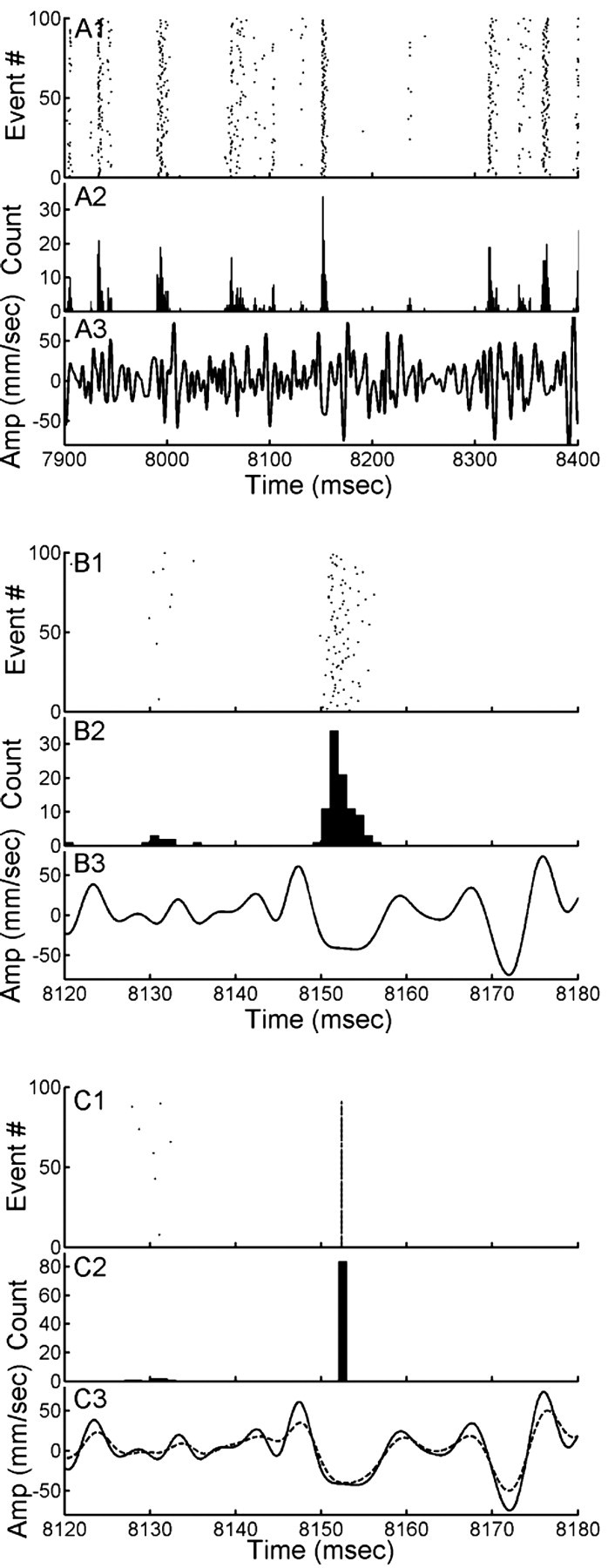
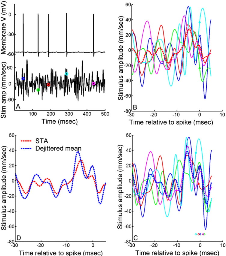
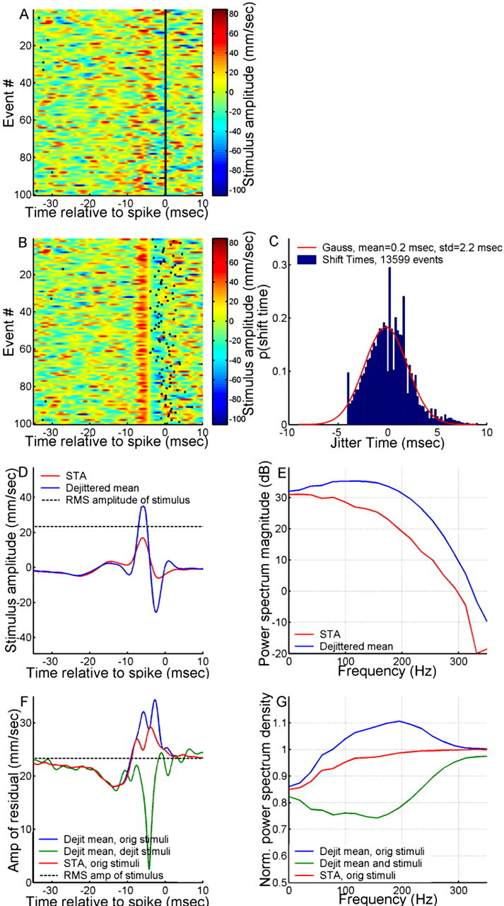
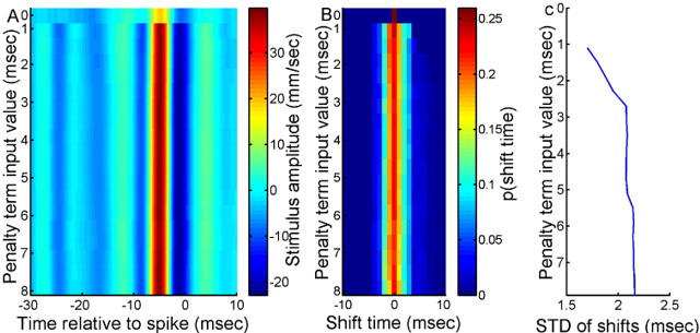
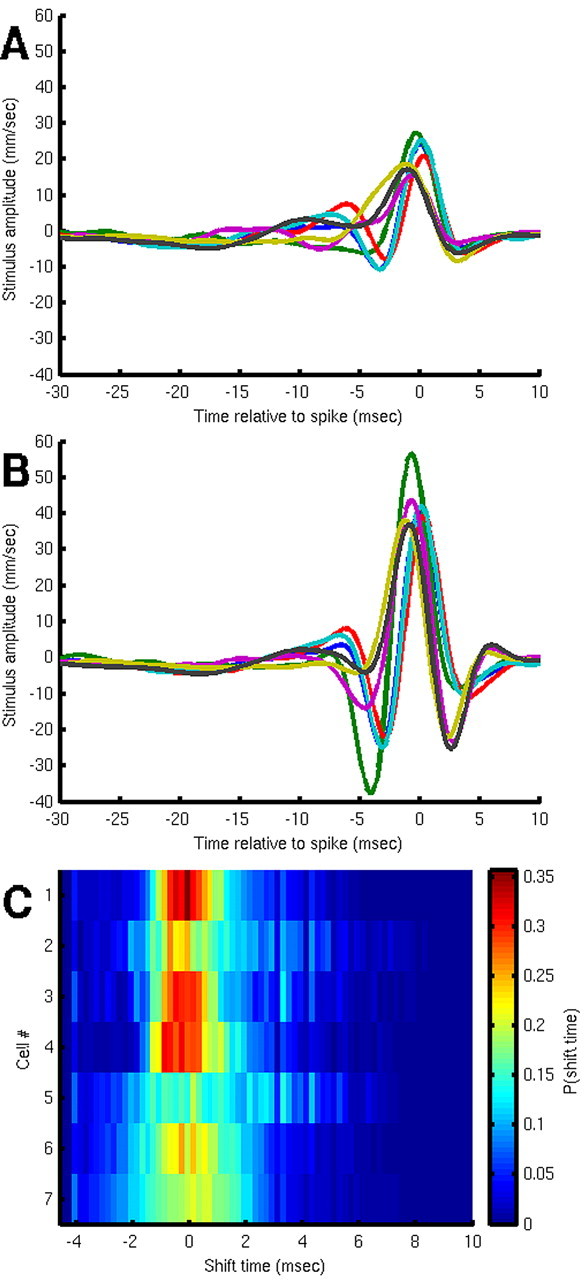
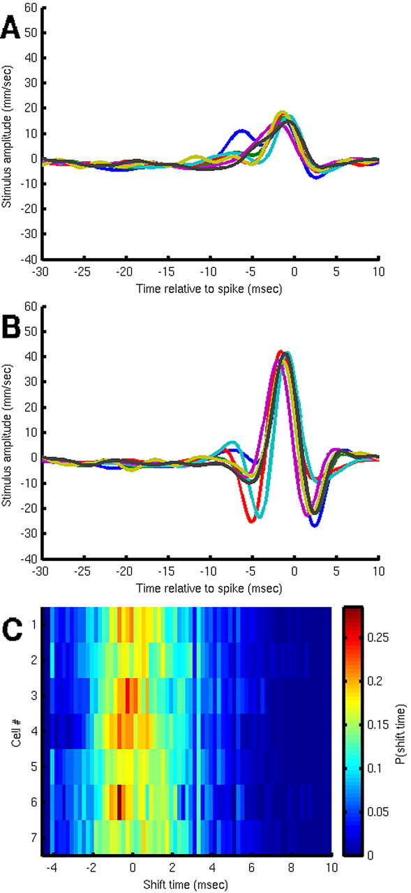
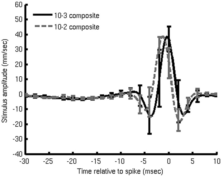
What is the meaning associated with a single action potential in a neural spike train? The answer depends on the way the question is formulated. One general approach toward formulating this question involves estimating the average stimulus waveform preceding spikes in a spike train. Many different algorithms have been used to obtain such estimates, ranging from spike-triggered averaging of stimuli to correlation-based extraction of "stimulus-reconstruction" kernels or spatiotemporal receptive fields. We demonstrate that all of these approaches miscalculate the stimulus feature selectivity of a neuron. Their errors arise from the manner in which the stimulus waveforms are aligned to one another during the calculations. Specifically, the waveform segments are locked to the precise time of spike occurrence, ignoring the intrinsic "jitter" in the stimulus-to-spike latency. We present an algorithm that takes this jitter into account. "Dejittered" estimates of the feature selectivity of a neuron are more accurate (i.e., provide a better estimate of the mean waveform eliciting a spike) and more precise (i.e., have smaller variance around that waveform) than estimates obtained using standard techniques. Moreover, this approach yields an explicit measure of spike-timing precision. We applied this technique to study feature selectivity and spike-timing precision in two types of sensory interneurons in the cricket cercal system. The dejittered estimates of the mean stimulus waveforms preceding spikes were up to three times larger than estimates based on the standard techniques used in previous studies and had power that extended into higher-frequency ranges. Spike timing precision was approximately 5 ms.

Figure 1.

A thought experiment to define the jitter problem using simulated recordings. A, Top trace, A segment of simulated stimulus consisting of three identical optimal features presented at random intervals, with no background noise. Bottom trace, Three spikes elicited by those stimulus features. B, Superposition of 500 examples of the stimulus waveform at an expanded timescale, with a raster plot of the jittered occurrence times of spike selicited by those 500 repetitions, and a histogram of those times immediately below. C, A total of 24 randomly selected samples of the stimulus wave form of the total data set of 500. These stimulus segments have been shifted with respect to one another to bring all of their elicited spikes into alignment (i.e., the vertical line to the lower right of the set of waveforms is the realigned spike raster). The mean of all realigned waveforms (i.e., the STA) is shown with the solid line. D, Comparison of the STA from C (solid line) with the actual stimulus waveform from B (gray line) and the dejittered mean (dotted trace).

Figure 2.

An experiment to illustrate the jitter problem, using a mechanosensory interneuron. A1, Raster of the spike times elicited by 100 repetitions of this waveform. A2, Histogram of this raster plot using 1 ms time bins. A3, A 0.5 s segment of the Gaussian noise stimulus waveform. B, The central 60 ms segment of the data shown in A at an expanded time scale. C1, Spike-time raster plot after realignment of the spikes in the distribution shown in B. C3, Dashed line, Mean of all stimulus segments realigned to the evoked spikes (i.e., the STA). C3, Solid line, The actual stimulus waveform (as in B). Amp, Amplitude.

Figure 3.

Illustration of the dejittering algorithm. A, A 500 ms segment of stimulus (bottom trace) and corresponding intracellular membrane potential with five spikes elicited by that stimulus (top trace). The time of spike occurrences are marked on the stimulus waveform with colored circles. Stim amp, Stimulus amplitude. B, Five 35 ms segments of the stimulus waveforms preceding each of the five spikes in A, locked to the times of spike occurrence at t = 0 ms. The color of each stimulus waveform matches the colored markers in A. The mean (i.e., spike-triggered average) waveform is shown with the dashed red line. C, The same five 35 ms segments, as shown in B, but now dejittered. The time-shifted spike times are shown by the markers under the waveforms. The mean is shown with the dashed blue line. D, Comparison of dejittered mean (blue dashed trace) with STA (red dashed trace) for the data.

Figure 4.

Characteristics of a dejittered mean stimulus. A, Random representative subset of 100 sample segments of stimulus-response data aligned to time of spike occurrence. The vertical black line at t = 0 is the raster plot of spikes superimposed on the color-coded traces of air-current velocity versus time. B, The same random subset of 100 segments of stimulus-response data from A but now dejittered so that their alignment is based on minimal variance of the stimuli. C, Shift times for all 13,600 samples (blue histogram) compared with a Gaussian having an STD of 2.2 ms (red line). D, STA (red trace) and dejittered mean (blue trace). The RMS amplitude of the stimulus is indicated with the dashed black line. E, Power spectra of the STA (red trace) and dejittered mean stimulus (blue trace). F, Red trace, Mean-square residual between the STA and the original (orig) stimulus segments. Blue trace, Mean-square residual between the dejittered (Dejit) mean and the original stimulus segments. Green trace, Mean-square residual between the dejittered mean and the dejittered stimulus segments. The RMS amplitude (amp) of the stimulus is indicated with the dashed black line. G, Power spectra of the residuals, normalized by power spectra of stimulus segments. Colors and abbreviations are the same as in F.

Figure 5.

Dependence of the dejittered mean shape and σ_tf on σ_t0. A, Mean output stimulus for each value of input penalty term σ_t0. The top row (σ_t0 = 0) shows the original STA. B, Probability distributions of the output shift times at 1 ms resolution for each value of the penalty term σ_t0. The top row (σ_t0 = 0) shows the spike times before dejittering. The color scale has been truncated from a maximum value of p (shift time) = 1 at σ_t0 = 0, shift time = 0. C, STD of dejitter shift times (σ_tf) for each value of input penalty term σ_t0.

Figure 6.

Composite average stimulus waveforms for a sample of seven cells from class 10-3. A, Standard STAs. B, Dejittered means. C, Histograms of the shift times for the seven IN10-3 cells at an expanded time scale, with color coding for the fraction of samples shifted by the indicated time.

Figure 7.

Composite average stimulus waveforms for a sample of seven cells from class 10-2. A, Standard STAs. B, Dejittered means. C, Histograms of the shift times for the seven IN10-2 cells at an expanded time scale, with color coding for the fraction of samples shifted by the indicated time.

Figure 8.

Comparison of the composite average dejittered mean stimulus waveforms for seven examples of each of the cell classes 10-3 (solid black curve) and 10-2 (dashed gray curve). Error bars on each curve represent 1 SD across the corresponding sample.

References

1. Bacon JP, Murphey RK (1984) Receptive fields of cricket (Acheta domesticus) are determined by their dendritic structure. J Physiol (Lond) 352: 601-613. - PMC - PubMed
1. Berry MJ, Warland DK, Meister M (1997) The structure and precision of retinal spike trains. Proc Natl Acad Sci USA 94: 5411-5416. - PMC - PubMed
1. Borst A, Theunissen FE (1999) Information theory and neural coding. Nat Neurosci 2: 947-957. - PubMed
1. Bryant HL, Segundo JP (1976) Spike initiation by transmembrane current: a white-noise analysis. J Physiol (Lond) 260: 279-314. - PMC - PubMed
1. Bryant HL, Marcos AR, Segundo JP (1973) Correlations of neuronal spike discharges produced by monosynaptic connections and by common inputs. J Neurophysiol 36: 205-225. - PubMed
Publication types
LinkOut - more resources