Modeling analytical ultracentrifugation experiments with an adaptive space-time finite element solution of the Lamm equation

Abstract

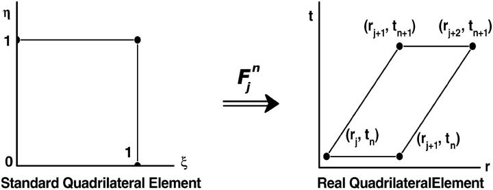
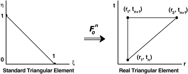
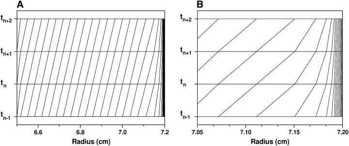
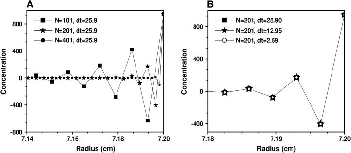
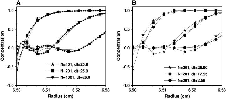
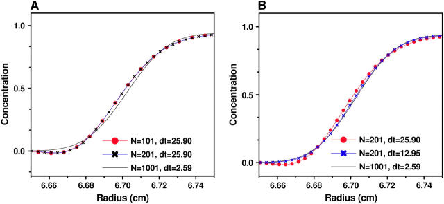
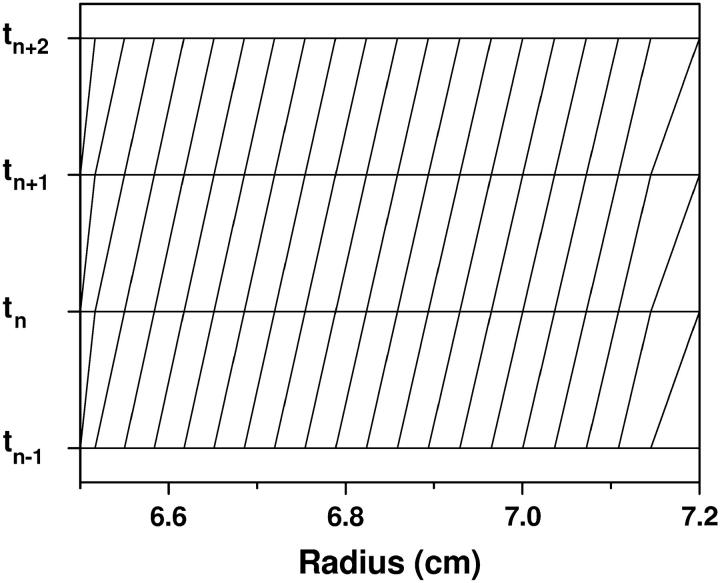
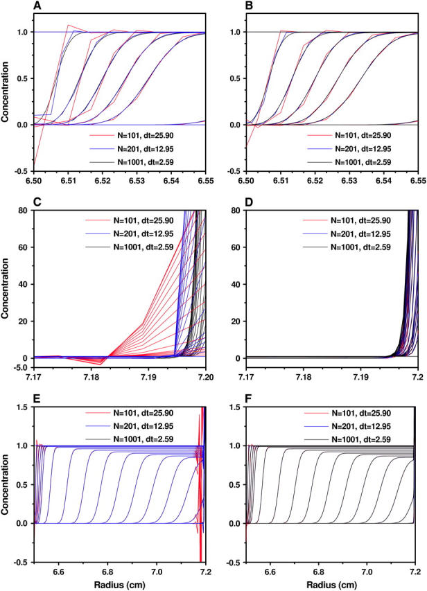
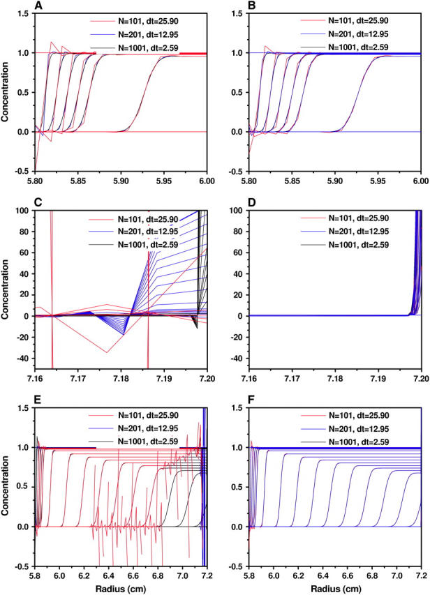
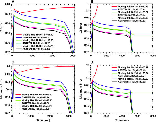
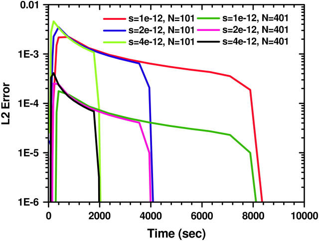
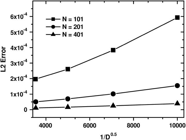
Analytical ultracentrifugation experiments can be accurately modeled with the Lamm equation to obtain sedimentation and diffusion coefficients of the solute. Existing finite element methods for such models can cause artifactual oscillations in the solution close to the endpoints of the concentration gradient, or fail altogether, especially for cases where somega(2)/D is large. Such failures can currently only be overcome by an increase in the density of the grid points throughout the solution at the expense of increased computational costs. In this article, we present a robust, highly accurate and computationally efficient solution of the Lamm equation based on an adaptive space-time finite element method (ASTFEM). Compared to the widely used finite element method by Claverie and the moving hat method by Schuck, our ASTFEM method is not only more accurate but also free from the oscillation around the cell bottom for any somega(2)/D without any increase in computational effort. This method is especially superior for cases where large molecules are sedimented at faster rotor speeds, during which sedimentation resolution is highest. We describe the derivation and grid generation for the ASTFEM method, and present a quantitative comparison between this method and the existing solutions.

FIGURE 1

Mapping Eq. 3 transforms the standard quadrilateral element into a quadrilateral element The finite element solution on is defined by transforming a bilinear function on with mapping

FIGURE 2

Mapping Eq. 5 transforms the standard triangular element into the triangular element The finite element solution on is defined by transforming a linear function on with mapping

FIGURE 3

ASTFEM grid point distribution for four successive time-steps. A shows the distribution for the entire cell, and in B a zoom of the region near the bottom is shown, clearly identifying the increased density of gridpoints at the bottom of the cell where the change of concentration is the largest and the highest resolution is needed.

FIGURE 4

Concentrations c(r, t) around the cell bottom obtained by Claverie's finite element method using (A) different numbers of grid points but the same time-step size, and (B) different time-step sizes but the same number of grid points. The parameters for this experiment are from Example 1, and t = 4922 s. From this figure it can be seen that the occurrence of oscillations at the bottom of the cell is strongly dependent on radial grid spacing, whereas a change of the time spacing has little influence.

FIGURE 5

Concentrations c(r, t) around the meniscus obtained by Claverie's finite element method using (A) different numbers of grid points but the same time-step size, and (B) different time-step sizes but the same number of grid points. The parameters for this experiment are from Example 1, and t = 25.9, 77.7, and 129.5 s. Here, the result is opposite to the effect shown in Fig. 4, and the oscillations near the meniscus are mostly influenced by the time discretization and only exist for the first several time-steps. Further reduction in the oscillation can be achieved by taking into account the rotor acceleration period at the beginning of the run.

FIGURE 6

Concentrations c(r, t) boundaries around the middle of the cell obtained by Claverie's finite element method using (A) different numbers of grid points but the same time-step size, and (B) different time-step sizes but the same number of grid points. The parameters for this experiment are from Example 1, and t = 518.0 s. In the middle of the cell the solution accuracy is affected by both the time and radial step size.

FIGURE 7

A typical grid used in the moving hat method for four successive time-steps. The radial distribution of the grid points is determined according to Eq. 16. The grid point density decreases toward the bottom of the cell, with the largest spacing at the bottom of the cell, where the highest resolution is actually needed.

FIGURE 8

Concentrations obtained by the moving hat method (A, C, and E) and the ASTFEM method (B, D, and F) with various N and δt for Example 1 (m = 6.5 cm, b = 7.2 cm, s = 10⁻¹², D = 2 × 10⁻⁷, 60,000 rpm, 9000 s). (A and B) The concentrations near the meniscus. (C and D) The concentrations near the bottom of the cell. (E and F) The concentrations on the entire cell. The largest difference can be noticed at the bottom of the cell (C and D), where the moving hat method is poorly conditioned. The oscillations near the meniscus are reduced for the ASTFEM method (A and B), and can be significantly reduced for both solutions when slow rotor acceleration is modeled in the solution.

FIGURE 9

Concentrations obtained by the moving hat method (A, C, and E) and the ASTFEM method (B, D, and F) with various N and δt for Example 2 (m = 5.8 cm, b = 7.2 cm, s = 1.562 × 10⁻¹², D = 1.279 × 10⁻⁷, 50,000 rpm, 6000 s). (A and B) The concentrations near the meniscus. (C and D) The concentrations near the bottom of the cell. (E and F) The concentrations on the entire cell.

FIGURE 10

Comparison of the evolution of the errors between the reference solution and the moving hat solutions or the ASTFEM solutions. (A and C) The L² error and the maximum error for the experiment setting in Example 1. (B and D) The L² error and the maximum error for the experiment setting in Example 2. Note that the ASTFEM solution achieves a lower error for all cases, and unlike the moving hat method, for N = 100 the ASTFEM solution remains stable and accurate.

FIGURE 11

The evolution of the L²-error in time for the ASTFEM solutions using N = 101 and 201 for experiments of various sedimentation coefficient s. Here the rotor speed was simulated at 50,000 rpm, D = 10⁻⁷, and m = 5.8, b = 7.2. This graph indicates that the accuracy of an ASTFEM solution does not depend much on the s values when the concentration boundary is in steady propagation. The same conclusion is true for Claverie's solution and the moving hat solution.

FIGURE 12

The averaged L²-error |c – c_ref| versus of the ASTFEM solution for experiments of various diffusion coefficient D. Here the rotor speed was simulated at 50,000 rpm, s = 10⁻¹², and m = 5.8, b = 7.2. This graph indicates that the accuracy of an ASTFEM solution increases as the diffusion coefficient D increases. The same conclusion is also true for Claverie's solution and the moving hat solution.

References

1. Lamm, O. 1929. The differential equation of the ultracentrifuge. Ark. Mat. Astron. Fys. 21B:1–4.
1. Claverie, J.-M., H. Dreux, and R. Cohen. 1975. Sedimentation of generalized systems of interacting particles. I. Solutions of systems of complete Lamm equations. Biopolymers. 14:1685–1700. - PubMed
1. Todd, G. P., and R. H. Haschemeyer. 1981. General solution to the inverse problem of the differential equation of the ultracentrifuge. Proc. Natl. Acad. Sci. USA. 78–11:6739–6743. - PMC - PubMed
1. Demeler, B., and H. Saber. 1998. Determination of molecular parameters by fitting sedimentation data to finite-element solutions of the Lamm equation. Biophys. J. 74–1:444–454. - PMC - PubMed
1. Schuck, P., C. E. MacPhee, and G. J. Howlett. 1998. Determination of sedimentation coefficients for small proteins. Biophys. J. 74–1:466–474. - PMC - PubMed
Publication types
Substances
LinkOut - more resources