History-dependent multiple-time-scale dynamics in a single-neuron model

Abstract

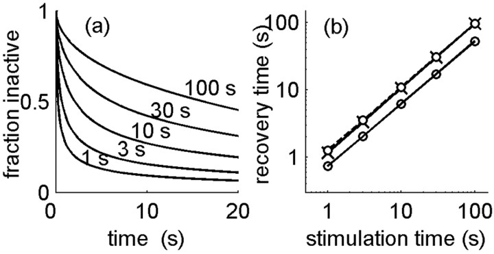
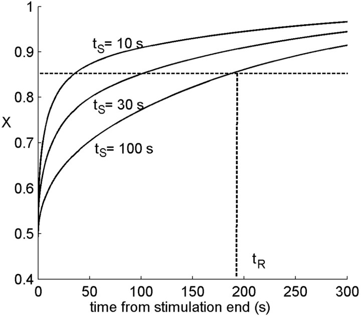
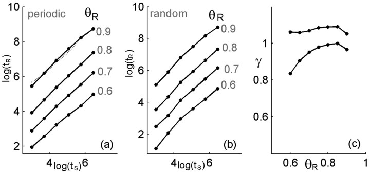
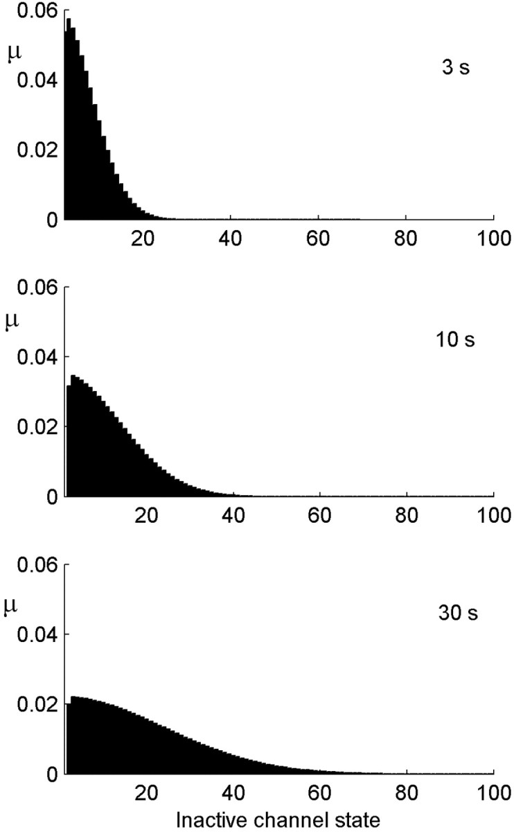
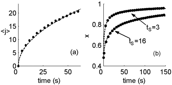
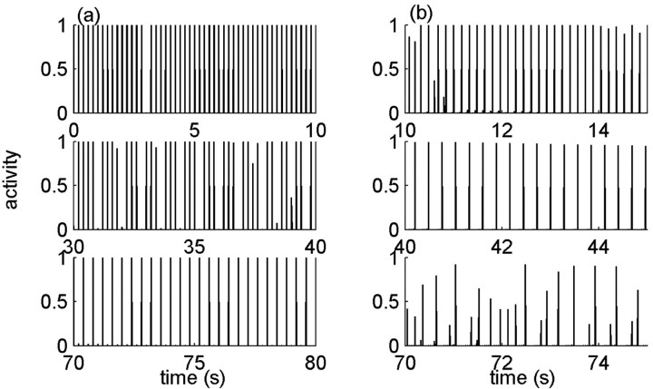
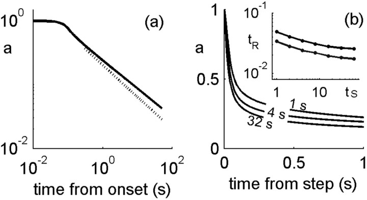
History-dependent characteristic time scales in dynamics have been observed at several levels of organization in neural systems. Such dynamics can provide powerful means for computation and memory. At the level of the single neuron, several microscopic mechanisms, including ion channel kinetics, can support multiple-time-scale dynamics. How the temporally complex channel kinetics gives rise to dynamical properties of the neuron is not well understood. Here, we construct a model that captures some features of the connection between these two levels of organization. The model neuron exhibits history-dependent multiple-time-scale dynamics in several effects: first, after stimulation, the recovery time scale is related to the stimulation duration by a power-law scaling; second, temporal patterns of neural activity in response to ongoing stimulation are modulated over time; finally, the characteristic time scale for adaptation after a step change in stimulus depends on the duration of the preceding stimulus. All these effects have been observed experimentally and are not explained by current single-neuron models. The model neuron here presented is composed of an ensemble of ion channels that can wander in a large pool of degenerate inactive states and thus exhibits multiple-time-scale dynamics at the molecular level. Channel inactivation rate depends on recent neural activity, which in turn depends through modulations of the neural response function on the fraction of active channels. This construction produces a model that robustly exhibits nonexponential history-dependent dynamics, in qualitative agreement with experimental results.

Figure 1.

Multiple time scales in a model of a membrane patch. a, Fraction of inactivated channels after a depolarizing voltage applied for various durations, plotted as a function of time from end of depolarization. Model parameters: β = 1 Hz; α₀ = 0.8 Hz. b, Characteristic time scale for recovery, defined by the decrease of inactivated fraction to a given threshold, plotted as a function of stimulation duration. These times obey a power-law scaling relationship with a power of ∼1. This scaling is weakly dependent on the choice of threshold for recovery (0.5 for top lines, crosses, and circles and 0.6 for bottom line). The same scaling is observed under cumulative inactivation; the dashed line with crosses shows the results for a periodic pulse train stimulus (25 Hz).

Figure 2.

Motivation for defining neuronal excitability. The normalized output firing rate is shown as a function of input current for the Hodgkin-Huxley model, with various values of the maximal conductances. Stimulus is a Gaussian noise with a correlation time of 500 ms (a) or 1 ms (b). Different values of the maximal conductances generally result in a different input/output function (a1, b1). In both curves, g_k = 30 μS/cm²; g_Na is changed between 90 μS/cm² (+) and 120 μS/cm² (diamonds). Changing the maximal conductance while keeping their ratio fixed (here 3) results in the same input/output function (a2, b2). g_k = 30 μS/cm² (+); g_k = 40 μS/cm² (diamonds). a3, b3, Dependence of the response threshold, defined as the input at half-maximal output, on the ratio of sodium to potassium maximal conductance.

Figure 3.

Closing the loop between neural activity and channel kinetics. a, Neural activity is characterized by a sigmoid rate function with a fixed width and a threshold that is modulated by neuronal excitability X. As excitability increases from 0 toward 1, the activity threshold decreases as θ_A = c_A/X. b, The effect of closing the loop on the dynamics of excitability: fraction of available ion channels as a function of time during stimulation in the neuron model (solid lines) compared with the model of a membrane patch (dashed, bottom line). In the neuron model, this fraction, the neural excitability, fluctuates around a steady-state value, X ≅ c_A. In the membrane patch, it continuously decreases with time as more and more channels are driven into inactivation.

Figure 4.

Stimulus, excitability, and neural response. A stimulus (s; top) is delivered to the model neuron. Activity (a; bottom) is elicited in response to the stimulus, according to a nonlinear response function (see Fig. 3a), which depends on the internal excitability variable (X; middle). a, Periodic unit pulses of width 10 ms and period 40 ms. b, Random stimulus, uniformly distributed in [0,1]. Parameters: α₀ = β = 20 Hz; σ = 0.1; c_A = 1/2.

Figure 5.

Recovery of excitability after a stimulation period. After stopping the stimulation, neuronal excitability slowly recovers back to its maximal value. Recovery is shown after stimulation of duration 10, 30, and 100 s. Note that recovery is nonexponential, and that although excitability starts from the same value, the time course is different depending on the history. Defining a typical time for recovery by a fixed threshold, this time t_R depends on history of stimulation and activity. Parameters: α_{0 [infi]} = β = 20 Hz; σ = 0.1; c_A = 1/2; stimulus frequency, 30 Hz.

Figure 6.

Scaling of recovery time with stimulation duration. Following the definitions of Figure 5, the time scale of recovery from inactivation shows a power-law scaling with stimulation duration t_R∼(t_S)^γ. Results for different choices of the recovery threshold are shown for a periodic train of stimulus pulses (a) and for a random Poisson pulse train with the same mean rate (b) averaged over realizations. The best fit for γ in the scaling function is shown for the two stimulus types in c and is between 0.8 and 1.05. Parameters: α₀ = β = 10 Hz; σ = 0.001; c_A = 1/2.

Figure 7.

Distribution of the channels among the inactive states after different stimulus durations. The distribution becomes broader as the stimulation duration increases. The population at the origin itself is stable at a value of ∼0.5 (data not shown). Parameters:α₀ =β = 20 Hz; σ = 0.1; c_A = 1/2.

Figure 8.

Diffusion approximation to channel dynamics. a, Mean of channel distribution among states, 〈j〉, as a function of stimulation time (circles). Although channel kinetics deviate from simple diffusion near the active state, the mean follows closely a diffusion-like behavior, , where t_S is the stimulation time (dashed line). b, Excitability as a function of time in the recovery phase, starting from the end of stimulation. Shown for comparison are the results of the numerical simulation (circles) and an analytic estimate based on the diffusion equation (dashed line; see Materials and Methods for details). Parameters: β = α₀ = 10 Hz; σ = 0.01; c_A = 1/2.

Figure 9.

Example of history dependence in the temporal pattern of response to stimuli. A periodic train of stimulus pulses is ongoing for a long time, and windows of response are chosen along the way for illustration. Model parameters here are: β = 1 Hz; α₀ = 30 Hz; σ = 0.001; c_A = 1/5. In this regimen, inactivation is strong and diffusive motion in the space of inactive states is very slow; the neural response is characterized by a hard threshold. a, Response to low frequency (5 Hz) starts by a one-to-one response (top), goes through an intermediate disordered response (middle), and then locks on a 1:2 response (bottom). b, In response to a high frequency of 25 Hz, the neuron responds only once every several pulses (top). The response frequency decreases at later times (middle) until the periodicity of the response breaks down completely (bottom).

Figure 10.

History-dependent multiple time scales in adaptation. a, Activity in the model neuron is plotted as a function of time from stimulus onset. Two regimens are seen; the tail decays approximately as t^-0.45 ( shown for comparison by a dashed line). b, Activity as a function of time since an abrupt change in stimulus strength from 0.6 to 1. For each line plotted, this time point in time was preceded by a different duration of the conditioning stimulus (1, 4, 32 s). At the switch to a higher stimulus, t = 0, the neuron responds with an increase in activity and then adapts nonexponentially with parameters that depend on the history. Inset, Time scale of decay, measured by threshold crossing for two values of the threshold, as a function of preceding stimulus duration. Here, β = α₀ = 10 Hz; σ = 0. 1; c_A = 1/2.

References

-
- Anderson JR (1995) Cognitive psychology and its implications. New York: Freeman.
- Bassingthwaighte JB, Liebovitch LS, West BJ (1994) Fractal physiology. New York: Oxford UP.
- Brenner N, de Ruyter van Steveninck RR, Bialek W (2000) Adaptive rescaling maximizes information transmission. Neuron 29: 695-702. - PubMed
- Carr DB, Day M, Cantrell AR, Held J, Scheuer T, Catterall WA, Surmeier DJ (2003) Transmitter modulation of slow, activity-dependent alterations in sodium channel availability endows neurons with a novel form of cellular plasticity. Neuron 39: 793-806. - PubMed
- de Ruyter van Steveninck RR, Zaagman WH, Masterbroek HAK (1986) Adaptation of transient responses of a movement-sensitive neuron in the visual system of the blowfly C. erythrocephala Biol Cybern 54: 223-236.
Publication types
MeSH terms
Substances
LinkOut - more resources
Full Text Sources