Simplified intersubject averaging on the cortical surface using SUMA

Abstract

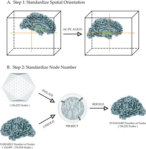
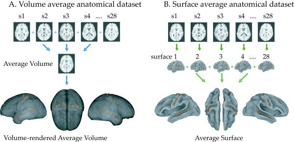
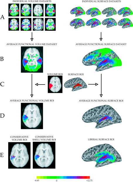
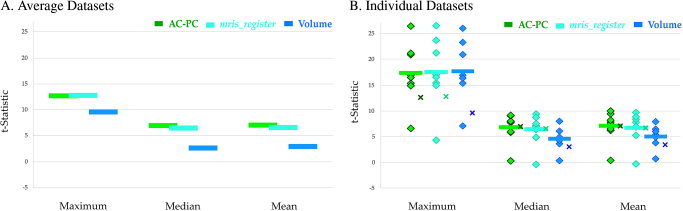
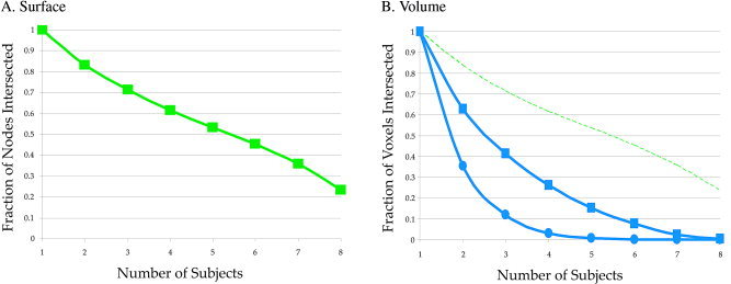
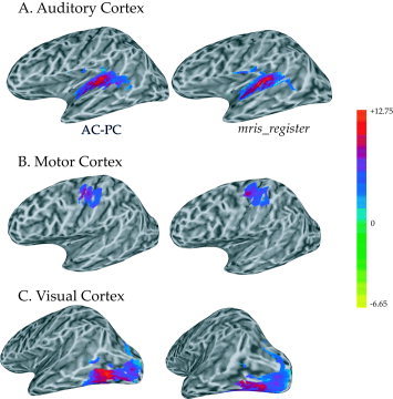
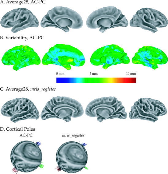
Task and group comparisons in functional magnetic resonance imaging (fMRI) studies are often accomplished through the creation of intersubject average activation maps. Compared with traditional volume-based intersubject averages, averages made using computational models of the cortical surface have the potential to increase statistical power because they reduce intersubject variability in cortical folding patterns. We describe a two-step method for creating intersubject surface averages. In the first step cortical surface models are created for each subject and the locations of the anterior and posterior commissures (AC and PC) are aligned. In the second step each surface is standardized to contain the same number of nodes with identical indexing. An anatomical average from 28 subjects created using the AC-PC technique showed greater sulcal and gyral definition than the corresponding volume-based average. When applied to an fMRI dataset, the AC-PC method produced greater maximum, median, and mean t-statistics in the average activation map than did the volume average and gave a better approximation to the theoretical-ideal average calculated from individual subjects. The AC-PC method produced average activation maps equivalent to those produced with surface-averaging methods that use high-dimensional morphing. In comparison with morphing methods, the AC-PC technique does not require selection of a template brain and does not introduce deformations of sulcal and gyral patterns, allowing for group analysis within the original folded topology of each individual subject. The tools for performing AC-PC surface averaging are implemented and freely available in the SUMA software package.

Figure 1

Two‐step process for creating standard individual subject surfaces. A: Spatial orientation is standardized by aligning the anterior and posterior commissures (AC and PC) to the center of standard space by translating and rotating the surface. An additional mid‐sagittal point (not shown) is used to define the plane. B: Node number is standardized by resampling to a projected standard icosahedron and refolding to the original space of the cortical surface model. When initially created, surface models contain variable numbers of nodes across subjects (left bottom). An icosahedron is tessellated to a standard number of nodes (left top). The icosahedron and the AC–PC aligned surface model are inflated to spheres (middle). The unfolded spherical representation of the surface model is mapped onto the inflated icosahedron, which is then refolded, resulting in a representation of the brain surface in its original state with a standard number of nodes (right).

Figure 2

Comparison of volume (A) and surface (B) intersubject averaging techniques with anatomical MR data. A: Whole‐brain anatomical scans from 28 subjects (top row) were transformed into standard space and the intensity was averaged in each voxel, creating a volume‐averaged anatomical dataset (middle row). A volume renderer was used to create a lateral view of the average left hemisphere, a top‐view of both hemispheres, and a lateral view of the right hemisphere (bottom row). Orange dashed lines indicate the approximate location of central sulcus and superior temporal sulcus. B: For the surface average, the same anatomical datasets were used to create cortical surface models (middle row). Each surface was then standardized (see Fig. 1) and the position of each node was averaged in space to create a surface‐average anatomical dataset (bottom row).

Figure 3

Comparison of volume (left column) and surface (right column) intersubject averaging techniques on BOLD fMRI data from auditory cortex. fMRI data (in color, overlaid on anatomical data, shown in gray scale) represents the t‐statistic of the contrast of the response to auditory vs. visual stimulation. Auditory cortex, in the planum temporale, shows a strong positive value for this contrast (red color, color scale shown at bottom of figure). A: Left: Functional datasets from each individual subject (n = 8) were Talairach transformed (slices shown at z = 10 mm). Right: Cortical surface models were created for each individual subject and functional data was mapped from the volume to the surface. B: Left: The average volume dataset was created by averaging the t‐statistic (for functional) or intensity (for anatomical) values at each location in Talairach space across subjects. Right: The average surface dataset was created by averaging the t‐statistic at each standardized node (displayed on an individual subject surface). C: A region of interest (ROI) for auditory cortex was created from the functional intersubject average volume and surface datasets. D: The auditory cortex ROI was applied to average volume (left) and surface (right) datasets. E: Alternative ROIs for comparison. Left: More conservative volume ROI created by surface gray‐white intersection algorithm. Middle: More conservative volume ROI created by cortical shell intersection algorithm. Right: Liberal surface ROI created by selecting all nodes intersecting the volume ROI in any of the individual subjects.

Figure 4

Statistical comparisons on functional data averaged with three different methods. A: The auditory cortex ROI was applied to surface and volume average datasets (see Fig. 3) and the maximum, median, and mean t‐statistics were calculated. The variability of each estimate was low: SD less than or equal to the thickness of each bar. Green symbols show the result of the AC–PC surface averaging method. Light blue symbols show the result of the mris_register surface averaging method [Fischl et al., 1999b]. Dark blue symbols show the volume average results. B: The surface average ROI was applied to each individual surface, and the volume average ROI was applied to each individual volume, generating maximum, median, and mean t‐statistics for each subject (same color scale as A). The average of these individual values (thick bars) provides an estimate of the ideal average value (assuming perfect intersubject alignment). This ideal value can be compared with the actual value obtained from surface and volume averages taken from A (shown with “x” symbols).

Figure 5

Correspondence of ROI constituents across subjects for surface (A) and volume (B) averages. A: The auditory cortex volume ROI (Fig. 3C, left) was intersected with the surface models from eight subjects, creating eight distinct surface ROIs. The proportion of nodes found in multiple individual subjects was tallied (100% of nodes found in at least one subject, 22% of nodes found in all eight subjects). B: The auditory cortex surface ROI (Fig. 3C, right) was intersected with the volume datasets of eight subjects, creating eight distinct volume ROIs. The proportion of Talairach locations found in multiple individual subjects was tallied. Volume ROIs calculated with a gray‐white matter intersection algorithm (blue circles) and a cortical shell intersection algorithm (blue squares). Surface ROI from A shown for comparison (dashed green line).

Figure 6

Auditory (A), motor (B), and visual (C) cortex ROIs applied to functional averages created with two surface‐averaging techniques, AC–PC and mris_register. A: Surface ROIs for auditory cortex generated with AC–PC alignment (left) and mris_register morphing (right). Colors represent t‐statistic of functional contrast (color bar at right, same for A, B, C). B: Surface ROIs for motor cortex. C: Surface ROIs for visual cortex.

Figure 7

Comparisons of anatomical averages created with two surface averaging techniques, AC–PC and mris_register. A: An average surface was created by averaging the location of each node across 28 subjects following AC–PC standardization. From left to right, left hemisphere (lateral and medial), right hemisphere (medial and lateral). B: The standard deviation between individual subjects and the average surface was calculated at each location on the surface and mapped to the average surface (color scale shows distance). C: Average surface created by averaging the same 28 subjects using mris_register standardization. D: Location of cortical poles following AC–PC (left) and mris_register (right) alignment. Temporal poles (green), occipital poles (red), and frontal poles (blue) were manually selected in each individual subject. The standard node index of each pole following registration is plotted on a spherical left hemisphere. Each spike (shown projecting normal to the surface for visibility) represents an individual subject.

References

1. Andrade A, Kherif F, Mangin JF, Worsley KJ, Paradis AL, Simon O, Dehaene S, Le Bihan D, Poline JB (2001): Detection of fMRI activation using cortical surface mapping. Hum Brain Mapp 12: 79–93. - PMC - PubMed
1. Beauchamp MS, Argall BD, Bodurka J, Duyn JH, Martin A (2004a): Unraveling multisensory integration: patchy organization within human STS multisensory cortex. Nat Neurosci 7: 1190–1192. - PubMed
1. Beauchamp MS, Lee KE, Argall BD, Martin A (2004b): Integration of auditory and visual information about objects in superior temporal sulcus. Neuron 41: 809–823. - PubMed
1. Buckner RL, Koutstaal W, Schacter DL, Rosen BR (2000): Functional MRI evidence for a role of frontal and inferior temporal cortex in amodal components of priming. Brain 123(Pt 3): 620–640. - PubMed
1. Chung MK, Worsley KJ, Paus T, Cherif C, Collins DL, Giedd JN, Rapoport JL, Evans AC (2001): A unified statistical approach to deformation‐based morphometry. Neuroimage 14: 595–606. - PubMed
Publication types