Sensitivity to interaural correlation of single neurons in the inferior colliculus of guinea pigs

Abstract

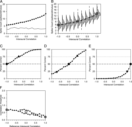
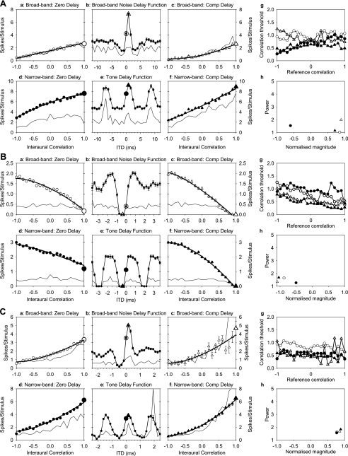
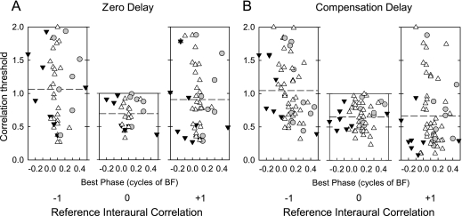
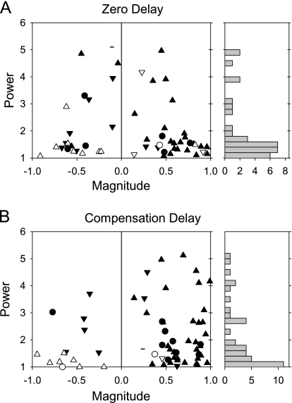
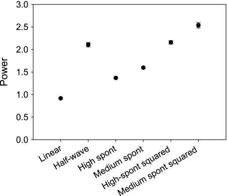
Sensitivity to changes in the interaural correlation of 50-ms bursts of narrowband or broadband noise was measured in single neurons in the inferior colliculus of urethane-anaesthetized guinea pigs. Rate vs. interaural correlation functions (rICFs) were measured using two methods. These methods compensated in different ways for the inherent variance in interaural correlation between tokens with the same expected correlation. The shape of all rICFs could be best described by power functions allowing them to be summarized by two parameters. Most rICFs were best fit by a power below 2, indicating that they were only slightly nonlinear. However, there were a few fitted functions that had a power of 3-6, indicating marked curvature. Modeling results indicate that the nonlinearity of the majority of rICFs was explicable in terms of the monaural transduction stages; however, some of the rICFs with power greater than 2 require either multiple inputs to the coincidence detector or additional nonlinearities to be included in the model. Discrimination thresholds were estimated at reference correlations of -1, 0, and +1 using receiver operating characteristic (ROC) analysis of the spike-count distribution at each correlation. Thresholds spanned the full possible range, from a minimum of 0.1 to the maximum possible of 2. Thresholds were generally highest with a reference correlation of -1, intermediate with a reference of 0, and lowest with a reference correlation of +1. Thresholds were lowest for the most steeply sloped rICFs, but thresholds were not strongly correlated to the spike rate variance. The lowest thresholds occurred using narrowband noise that was compensated for internal delays, but they were still about three times larger than human psychophysical thresholds measured using similar stimuli. The data suggest that, unlike pure tone interaural time difference, discrimination of a population measure is required to account for behavioral interaural correlation discrimination performance.

Fig. 1

Standard deviation of interaural correlation of noise samples (left axis) and human correlation discrimination threshold (right axis) as a function of interaural correlation. Open symbols show the standard deviation of the measured correlation of 500 noise tokens for two different bandwidth (W), duration (T) products (using first method of generation described in the section “Rate vs. Interaural correlation functions”). The solid line running between these points is the empirically fitted function , which follows the data well. A similar plot is shown in Gabriel and Colburn's (1981) Figure 6, although a less well fitting function is plotted, where it is noted that an analytical solution is difficult (p.1397). Human psychophysical interaural correlation discrimination thresholds are shown as solid circles joined by lines for 1-s long noise samples at 85 dB SPL (Pollack and Trittipoe, 1959a).

Fig. 2

Illustration of receiver operating characteristic (ROC) analysis. A Rate vs. interaural correlation function (rICF) as a solid line joined by circles. Variance of distribution of spike counts is shown as a light line. rICF was collected by using the second method of generation described in the section “Rate vs. Interaural correlation functions.” Fifty repeats each of 10 tokens were collected and the results pooled across tokens, so each point is the result of 500 measures. B rICF (joined symbols) with distribution of number of times each spike count occurred superimposed corresponding to filled symbols. The reference correlations −1, 0, and +1 used in panels C–E are encircled. C “Neurometric” function showing predicted percentage correct in a simulated 2IFC experiment (see the section “Receiver operating characteristic analysis” for details). The large circle shows the reference correlation of −1 and the large, upward triangle shows the correlation closest to the 75% threshold. D Same as in C, but for a reference correlation of 0. The large downward triangle shows the correlation closest to the 25% threshold. E Same as in D, but for a reference correlation of +1. FInteraural correlation thresholds as a function of reference correlation. Upward pointing triangles are the 75% correct thresholds and downward pointing triangles are the 25% correct thresholds. Circles show the threshold values reported in subsequent figures at references of −1, 0, and +1. The reported threshold at 0 is the mean of the 25% and 75% correct thresholds.

Fig. 3

Example analyses for: A a peak neuron with a CF of 127 Hz and a best phase of 0.14 cycles, “compensation” delay was 790 μs (0.1 cycle); B a trough neuron with a CF of 412 Hz and a best phase of 0.35 cycles, “compensation” delay was −850 μs (−0.15 cycles); C an asymmetrical neuron with a CF of 624 Hz and a best phase of 0.18 cycles, “compensation” delay was 160 μs (0.1 cycles). In all panels a–f, the error bars show the standard error of mean. (a, c, d, f) Interaural correlation functions (rICFs): the number of spikes elicited in 80 ms after onset of stimulus as a function of interaural correlation. The light line shows the variance of the spike count distribution. The thick line shows the fitted power function. The large symbol shows the stimulus condition that is equivalent to a condition within the delay function (b, e). The combinations of stimulus bandwidth and noise delay used are as follows: (a) broadband, zero noise delay; (c) broadband, “compensation” noise delay; (d) narrowband, zero noise delay; (f) narrowband, “compensation” noise delay. b Broadband noise delay function. The large circle emphasizes the zero-ITD condition, which can be compared with the circled condition in subpanel (a). The large triangle shows the “compensation” delay, which can be compared with the emphasized condition in subpanel (c). e Tone delay function. Large symbols as for (b). g Interaural correlation thresholds as a function of reference threshold for the four conditions shown in panels a, c, d, f. Symbols match the symbols in the individual panels: open circles = broadband, zero noise delay; open triangles = broadband, “compensation” noise delay; filled circles = narrowband, zero noise delay; filled triangles = narrowband, “compensation” noise delay. Thresholds shown are the average of the 25% and 75% correct thresholds. h Power and normalized magnitudes for the power function fits shown in panels a, c, d, f. Compare with Figure 11. Symbols are as in (g). The power function fitted in Ad and the solid circle in Ah are fitted with negative power function, all other fits are the positive power functions.

Fig. 4

Example analysis for an asymmetrical neuron with a CF of 354 Hz and a best phase of 0.34 cycles showing the effect of a large best phase upon the slope of the zero-delay rICFs. Symbols and format subpanels a–f are as in Figure 3.

Fig. 5

Correlation discrimination thresholds measured from the rICFs. A Narrowband zero-delay conditions. B Narrowband “compensation” delay conditions. Within each panel from left to right are shown the thresholds for discriminations away from correlations of −1, 0, and +1, respectively. Within each subpanel the thresholds are plotted as a function of neuron characteristic frequency. Symbols indicate the neuron type: open, upward triangles represent peak neurons (n = 34 and 41 for panels A and B, respectively); gray circles asymmetrical neurons (n = 8, 12); solid, downward triangles trough neurons (n = 13, 10). The dashed lines show the mean threshold averaged across all neuron types. For comparison, thresholds from a recent psychophysical study are shown: the thick solid lines show the human interaural correlation threshold interpolated to a duration of 50 ms with a bandwidth of 100 Hz, centred on 500 Hz, at 70 dB SPL (Bernstein and Trahiotis, 1997); threshold for a reference correlation of −1 was not measured. For reference correlations of ±1, the maximum possible threshold is 2, which corresponds to the first discriminable point being at the opposite end of the function. The maximum threshold for a reference of 0 is only 1, because thresholds were measured from 0 towards either +1 or −1.

Fig. 6

A, B Comparison of correlation threshold at a reference correlation of +1 and the standard deviation of normalized rICF at a correlation of +1. C, D Comparison of correlation threshold at a reference correlation of +1 and the inverse of the slope of the rICF at a correlation of +1 derived from the product of the magnitude and power of the power curve fitted to the rICF normalized by the maximum firing rate (see the section “Interaural correlation discrimination thresholds” for further details). A, C Results for zero delay (n = 28, 8, and 9 for peak, asymmetrical, and trough neurons, respectively). B, D Results for “compensation” delay (n = 40, 11, and 8 for peak, asymmetrical, and trough neurons, respectively). The solid lines are linear regression fits and the correlation coefficients are shown in each panel. Symbols are as in Figure 5.

Fig. 7

Same as in Figure 5, except that results are plotted as a function of neuron best phase.

Fig. 8

Comparison of correlation thresholds measured in the same neurons for zero-delay conditions (ordinate) and for “compensation” delay conditions (abscissa) for A narrowband and B broadband stimuli. From left to right, subpanels show thresholds for −1, 0, and +1 reference correlations, respectively. Diagonal line represents equality. Symbols are as in Figure 5, except that crosses mark thresholds of neurons where the “compensation” delay was zero. The numbers of neurons where the “compensation” delay waszero in each panel was: A 11, 8, 12; B 7, 5, 7 (from left to right). Thenumber of peak neurons shown are: A 6, 4, 7; B 3, 2, 3. Troughneurons: A 4, 3, 5; B 3, 4, 4. Asymmetrical neurons: A 5, 6, 7; B 4, 2, 6.

Fig. 9

Comparison of correlation thresholds measured in the same neurons for broadband stimuli (ordinate) and narrowband stimuli (abscissa) for A zero-delay conditions and B “compensation” delay conditions. From left to right subpanels show thresholds for −1, 0, and +1 reference correlations, respectively. Diagonal line represents equality. Symbols are as in Figure 5. The number of peak neurons shown are: A 13, 21, 15; B 8, 8, 9 (from left to right). Trough neurons: A 5, 7, 6; B 7, 6, 7. Asymmetrical neurons: A 5, 8, 7; B: 5, 4, 5.

Fig. 10

The power (p) and normalized magnitude (m) of power curves (y(x′) = a + bx′^p) fitted to the unnormalized rICFs for A zero-delay conditions and B “compensation” delay conditions. The distributions to the side of each plot show histograms of the fitted powers. Symbols are as in Figure 5, but with the shading altered: black symbols show curves fitted with the ordinary power function (x′ is (1 + x)/2), which have their steepest section at a correlation of +1, whereas the white symbols were fitted with negative power functions (x′ is (1 − x)/2), with their steepest part at a correlation of −1. The functions were normalized by the maximum of the fitted function, which differed depending on the sign of b. If b is positive, then the maximum of the function occurred at x′ = 1 and is a + b, so where m = b / (a + b). If b is negative, then the maximum is at x′ = 0 and is a, so where m = b/a. In both of these equations m represents the magnitude of the function, i.e., the amount by which it changes from correlations of −1 to +1, and the baseline value can be determined as 1 or (1 −m) depending upon the sign of m. If m is positive, then the function increases with increasing x′, whereas if m is negative then it decreases with increasing x′. In panel A, there are 44 neurons for which a positive power function was the better fit, comprising 25 peak neurons, 7 asymmetrical neurons and 8 trough neurons. There were 14 neurons for which a negative power function was the better fit, comprising 9 peak neurons, 1 asymmetrical neuron, and 4 trough neurons. In panel B there are 53 neurons for which a positive power function was the better fit, comprising 34 peak neurons, 9 asymmetrical neurons, and 9 trough neurons. There were 11 neurons for which a negative power function was the better fit, comprising 7 peak neurons, 3 asymmetrical neuron, and 1 trough neuron.

Fig. 11

Power of curves fitted to simulated rICFs. The model is described in the section “Shapes of the rate vs. interaural correlation functions.” The abscissa shows the type of peripheral transduction used before input to a coincidence detector (which multiplied together its inputs and summed the result over the duration of the stimulus). Linear: the inputs to the coincidence detector were just the signal filtered by a basilar membrane filtering stage. Half-wave: the same as in linear, except that the signals were half-wave-rectified before input to the coincidence detector. High spont: the same as in linear, except that the stimulus was passed through a simulation of high-spontaneous rate auditory nerve fibers (Meddis et al. 1990). Medium spont: the same as in high spont, except that the simulation was for a medium spontaneous rate fiber. High spont squared: the same as in high spont, except that the auditory nerve output was squared before input to the coincidence detector to simulate two similar inputs from each side. Medium spont squared: the same as in High spont squared, except that the simulation was for a medium spontaneous rate fiber. The error bars show the standard error from 10 repeats.

References

1. Akeroyd MA. A binaural cross-correlogram toolbox for MATLAB. http://www.ihr.gla.ac.uk/products/matlab/ (computer software), 2004.
1. {'text': '', 'ref_index': 1, 'ids': [{'type': 'PubMed', 'value': '8989405', 'is_inner': True, 'url': 'https://pubmed.ncbi.nlm.nih.gov/8989405/'}]}
2. Albeck Y, Konishi M. Responses of neurons in the auditory pathway of the barn owl to partially correlated binaural signals. J. Neurophysiol. 74:1689–1700, 1995. - PubMed
1. {'text': '', 'ref_index': 1, 'ids': [{'type': 'DOI', 'value': '10.1007/s10162-004-4027-4', 'is_inner': False, 'url': 'https://doi.org/10.1007/s10162-004-4027-4'}, {'type': 'PMC', 'value': 'PMC2504554', 'is_inner': False, 'url': 'https://pmc.ncbi.nlm.nih.gov/articles/PMC2504554/'}, {'type': 'PubMed', 'value': '15492883', 'is_inner': True, 'url': 'https://pubmed.ncbi.nlm.nih.gov/15492883/'}]}
2. Batra R, Yin TCT. Cross correlation by neurons of the medial superior olive: A reexamination. J. Assoc. Res. Otolaryngol. 5:238–252, 2004. - PMC - PubMed
1. {'text': '', 'ref_index': 1, 'ids': [{'type': 'PubMed', 'value': '9310415', 'is_inner': True, 'url': 'https://pubmed.ncbi.nlm.nih.gov/9310415/'}]}
2. Batra R, Kuwada S, Fitzpatrick DC. Sensitivity to interaural temporal disparitites of low- and high-frequency neurons in the superior olivary complex. II. Coincidence detection. J. Neurophysiol. 78:1237–1247, 1997. - PubMed
1. {'text': '', 'ref_index': 1, 'ids': [{'type': 'DOI', 'value': '10.1121/1.419863', 'is_inner': False, 'url': 'https://doi.org/10.1121/1.419863'}, {'type': 'PubMed', 'value': '9265758', 'is_inner': True, 'url': 'https://pubmed.ncbi.nlm.nih.gov/9265758/'}]}
2. Bernstein LR, Trahiotis C. The effects of randomizing values of interaural disparities on binaural detection and on discrimination of interaural correlation. J. Acoust. Soc. Am. 102:1113–1120, 1997. - PubMed
LinkOut - more resources