A guideline for analyzing circadian wheel-running behavior in rodents under different lighting conditions

Abstract

Most behavioral experiments within circadian research are based on the analysis of locomotor activity. This paper introduces scientists to chronobiology by explaining the basic terminology used within the field. Furthermore, it aims to assist in designing, carrying out, and evaluating wheel-running experiments with rodents, particularly mice. Since light is an easily applicable stimulus that provokes strong effects on clock phase, the paper focuses on the application of different lighting conditions.

Fig. 1. Schematic single and double plotted actograms and masking. (A)

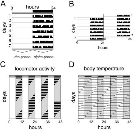
Wheel-running activity is plotted as an actogram with each horizontal line corresponding to one day. Black vertical bars plotted side-by-side represent the activity, or number of wheel revolutions. The height of each vertical bar indicates the accumulated number of wheel revolutions for a given interval (e.g. 5 min). The rho- and alpha-phase marked at the bottom of the actogram refer to rest and activity, respectively. The white and black bar at the top of the scheme depicts light (12 h) and darkness (12 h), respectively. (B) To better visualize behavioral rhythms, actograms are often double plotted by aligning two consecutive days horizontally (e.g. day 1 left and day 2 right). (C) Schematic actogram of a nocturnal animal kept in very short photoperiods (LD 6:6). Since the animal is only showing activity during the dark phases it seems to entrain to the prevailing LD cycle. (D) Parallel monitoring of body temperature reveals that this apparent entrainment is only masking. Although the readout parameter "activity" seemingly adapts to the new schedule, body temperature continues to cycle with its free-running period length implicating that the circadian clock of the animal is not entrained. LD, light-dark cycle.

Fig. 2. Transients and Aftereffects.

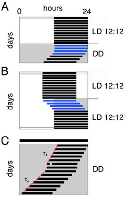
Transients (blue bars) can be caused by various treatments, such as the release of the animal into constant conditions (A) or a shift in the lighting regime (B). These transients usually persist for several days depending on the strength of the provoking signal. The white and black bar at the top of the scheme depicts light (12 h) and darkness (12 h), respectively. (C) An animal kept in constant darkness (DD) displays a stable free-running rhythm with a period length τ₁ before it is subjected to a light pulse. This pulse leads to a phase shift and often provokes τ₂, which is different from τ₁, as an aftereffect. If the animal is left in DD long enough after this treatment, it will again display its old period length τ₁. The red regression lines are drawn through the onsets before and after the light pulse to determine τ₁ and τ₂, respectively. The black bar at the top of the scheme represents constant darkness (24 h) conditions. DD, constant darkness; LD, light-dark cycle.

Fig. 3. T-cycles.

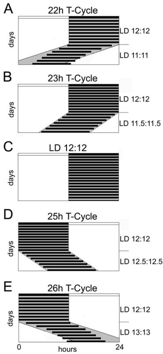
T-cycles are LD cycles with a period length other than 24 hours (T = L + D). Mice are able to entrain to T-cycles of 23 (B) and 25 (D) hours but not to T-cycles of 22 (A) and of 26 (E) hours. Panel C represents a normal 24 hours LD 12:12 cycle. All schemes are plotted on 24 hours scale where the white area represents lights on and the gray area lights off, respectively. The white and black bar at the top of the scheme depicts light and darkness of the LD 12:12 cycle the animals were entrained to in the beginning of each panel. Each species has a distinct range of entrainment; the schemes here represent the range for mice. The black horizontal bars display the active time of the animals. LD, light–dark cycle; T, period or cycle time of a Zeitgeber; h, hours.

Fig. 4. Schematic representation of external time (ExT) in photoperiods and T-cycles.

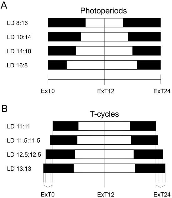
External time (ExT) subdivides any light-dark cycle into 24 units using the following formula: number of hours*24/T elapsed since the middle of the dark period. ExT0 (= ExT24) is determined as the middle of the dark period. ExT12 corresponds to the middle of the light phase. Vertical black lines indicate the corresponding external time. Black bars represent the dark period whereas the white bars correspond to lights on. (A) Schematic representation of ExT for photoperiods. (B) Schematic representation of ExT for T-cycles. ExT, external time; LD, light–dark cycle; T, period or cycle time of a Zeitgeber; h, hours.

Fig. 5. Real actograms and phase response curve (PRC). (A)

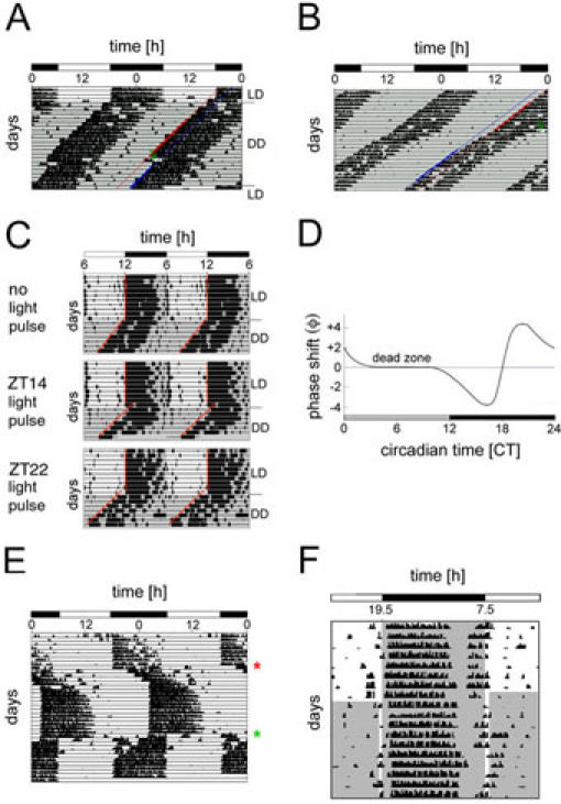
Plot of mouse locomotor activity before and after administering a light pulse (LP) at CT14 provoking a phase delay. The mouse was entrained to an LD 12:12 cycle before it was released into constant darkness (DD). The line above “DD” indicates the transition from LD to DD. When a stable free-running rhythm was established, a LP (green arrow) was administered at CT14 for 15 min. In order to quantify the phase shift, regression lines are drawn through 10 activity onsets before (red) and through 6 onsets after (blue) the LP. The horizontal distance between them corresponds to the phase shift triggered by the LP. (B) Plot of mouse locomotor activity before and after administering a LP at CT22 provoking a phase advance. The mouse was entrained to LD 12:12 (not shown) and then released into DD. As soon as a stable free-running rhythm was established, a LP (green arrow) was administered at CT22 for 15 min. In order to quantify the phase shift, regression lines are drawn through 6 activity onsets before (red) and through 7 onsets after (blue) the LP. The horizontal distance between them corresponds to the phase shift triggered by the LP. (C) Typical actograms of wild-type mice subjected to an Aschoff type II protocol. Mice were entrained to an LD 12:12 cycle (10 days) before releasing them into DD. The line above “DD” indicates the transition from LD to DD. The grey background represents darkness. Upon release into DD, no light pulse was administered to the mouse in the upper panel, whereas light pulses of 15 min were applied to the mouse at ZT14 (middle panel) and ZT 22 (lower panel). Regression lines (red) are drawn through the onsets of wheel-running activity in order to calculate the phase shift. Adapted from (26). (D) Typical light phase response curve (PRC) for nocturnal rodents. The grey and black bars below the PRC indicate subjective day and night, respectively. The X-axis shows the circadian time (CT) at which the light pulse was applied whereas the Y-axis displays the observed phase shift (f) [h]. Light pulses administered between CT11 and CT18 provoke a phase delay (negative values). Light pulses between CT19 and CT3, on the other hand, generate phase advances (positive values). Between CT4 and CT10, no phase shift can be observed (dead zone). (E) Jet lag can be mimicked in the lab by subjecting entrained animals to a rapid shift in the lighting schedule. This actogram shows the locomotor behavior of a mouse that was first entrained to LD 12:12 with light from 6 am to 6 pm. After 10 days, the lighting schedule was still LD 12:12 but shifted to "lights on" at 2 pm and "lights off" at 2 am (red star). The mouse only entrains after around 7 days of transition to the new LD cycle. 17 days after the first shift, the lighting schedule was again shifted to the original schedule (LD 12:12 from 6 am to 6 pm; green star). (F) Panel F shows an actogram of a mouse subjected to a skeleton photoperiod. The mouse was first entrained to LD 12:12 with lights on from 7:30 am to 7:30 pm for 8 days. The grey background represents lights off, whereas the white area stands for lights on. After day 8, an asymmetrical skeleton photoperiod was applied with a shorter pulse in the evening (dusk) and a longer one in the morning (dawn). Due to the two light pulses, the mouse remains entrained and wheel-running activity does not differ tremendously compared to LD 12:12. Adapted from ref. 31. LD, light-dark cycle; h, hours; DD, constant darkness.

Fig. 6. Wheel-running cages and isolation cabinets. (A)

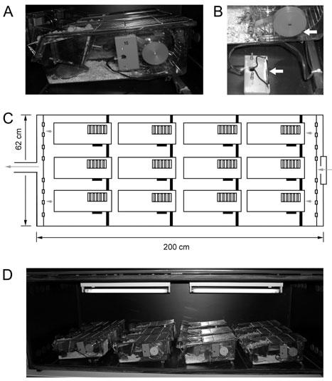
Individually housed mouse in a wheel-running cage connected via a magnetic switch to the system recording wheel revolutions. On each rotation of the running wheel, the magnetic switch is once opened and closed. (B) Detailed view of the magnet (upper arrow) and the magnetic switch (lower arrow). (C) Schematic representation of a ventilated isolation cabinet (200 x 62 cm) offering space for 12 wheel-running cages. The arrows represent the airflow through the cabinet. (D) Picture of a fully occupied isolation cabinet with two light bulbs at the ceiling.

Fig. 7. Adaptation time and CT diagram. (A)

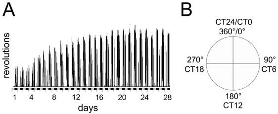
Linear recording of wheel-running activity of a male wild type mouse (C57BL/6 x 129SV) under LD 12:12 conditions. Without prior wheel-running experience mice need two to three weeks to fully develop their wheel-running capacity. Only after this initial training (and entraining) phase experimental manipulations should be applied (X-axis: days of experiment; Y-axis wheel revolutions; black and white bars indicate dark and light phases, respectively; bin size for activity counts is 6 min). (B) Diagram comparing circadian time (CT) in degrees versus CT units.

Fig. 8. Impact of constant darkness on weight and overall activity of wild-type mice. (A)

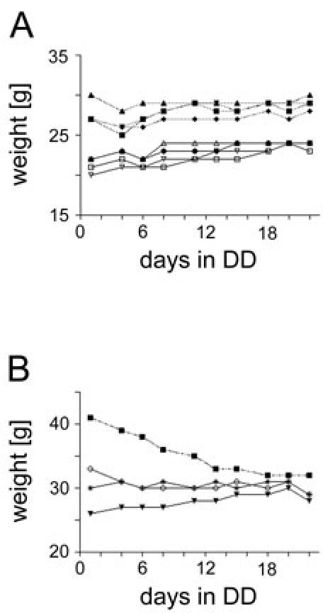
Weight curves of 8 littermates (males: solid lines / females: hatched lines) with a mixed C75BL/6 x 129S5/SvEvBrd background. Mice were reared in a normal LD 12:12 cycle and then transferred to constant darkness (DD). They were housed individually in wheel-running cages where food and water were accessible ad libitum. During 22 days, they were weighed regularly using night vision goggles. The x-axis displays the days spent in constant darkness whereas the y-axis displays the weight [g]. (B) Weight curves of 4 male mice with a 129SvEvBrd/129Ola background. Only one mouse (black square) that was overweight in the beginning looses weight during monitoring.

References

-
- Dunlap JC, Loros JL, DeCoursey PJ. CHRONOBIOLOGY – biological timekeeping. Sinauer Associates. 2004;3(24):67–105.
- Pittendrigh CS. On the mechanism of the entrainment of a circadian rhythm by light cycles. In: Circadian clocks; edited by: Aschoff J, Amsterdam: Elsevier (1965); 277-297.
- Pittendrigh CS. Circadian systems: entrainment. In: Handbook of behavioral neurobiology, Vol. 4 Biological Rhythms, edited by Aschoff J, New York: Plenum Press (1981); 95-124.
- Pittendrigh CS, Daan S. A functional analysis of circadian pacemakers in nocturnal rodents. IV. Entrainment: Pacemaker as clock. J Comp Physiol A. 1976;106:291–331.
- Aschoff J, Daan S, Honma KI. Zeitgeber, entrainment, and masking: some unsettled questions. In: Vertebrate Circadian System (Structure and Physiology), edited by Aschoff J, Daan S, Gross GA, Berlin: Springer-Verlag (1982); 13-24.
LinkOut - more resources
Full Text Sources
Other Literature Sources