Evidence of a large-scale functional organization of mammalian chromosomes

Abstract

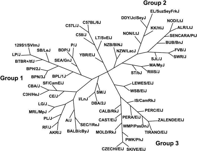
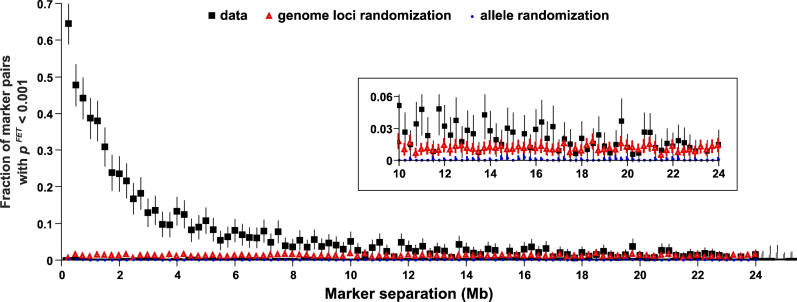
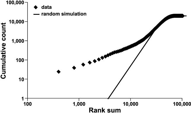
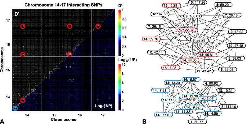
Evidence from inbred strains of mice indicates that a quarter or more of the mammalian genome consists of chromosome regions containing clusters of functionally related genes. The intense selection pressures during inbreeding favor the coinheritance of optimal sets of alleles among these genetically linked, functionally related genes, resulting in extensive domains of linkage disequilibrium (LD) among a set of 60 genetically diverse inbred strains. Recombination that disrupts the preferred combinations of alleles reduces the ability of offspring to survive further inbreeding. LD is also seen between markers on separate chromosomes, forming networks with scale-free architecture. Combining LD data with pathway and genome annotation databases, we have been able to identify the biological functions underlying several domains and networks. Given the strong conservation of gene order among mammals, the domains and networks we find in mice probably characterize all mammals, including humans.

Figure 1. Neighbor-Joining Distance Tree of the Mouse Strains Used in This Study

The length and angles of the branches have been optimized for printing and do not represent actual phylogenetic distances. Group 1, Bagg albino, 129, and DBA-related strains; group 2, Swiss mice and Asian strains; group 3, wild-derived strains.

Figure 2. Dependence of the Fraction of Markers in LD from the Distance between Them

Fisher's exact test was used, p_FET < 0.001 unadjusted. Solid squares, actual data; red triangles, randomized genomic positions of the markers; solid circles, randomized alleles and strains.

Figure 3. A Representation of LD between Marker Pairs on Mouse Chromosome 14 Reveals a Domain Structure

LD is plotted as D′ and log₁₀ (1/p_FET) above and below the diagonal, respectively. The x- and y-coordinates are NCBI Build 33 genome positions for SNPs. Black regions reflect genomic sequence not covered in this SNP set (i.e., missing data). To highlight pairs of interest, D' values have been suppressed (plotted as gray) for marker pairs with p_FET > 10⁻³. White boxes represent LD domains, identified as described in the text. Yellow boxes represent regions of synteny identified through mouse-rat-human-chicken comparison [19].

Figure 4. Distribution of Sum of Rank Scores for Marker Pairs

Distribution is shown for the three groups of mouse strains as described in Materials and Methods. Deviation from the random simulation indicates sharing of LD pairs between groups.

Figure 5. An Example of a Gene Network that Is Largely Contained within an LD Domain Located between 167.2 and 174.2 Mb on Mouse Chromosome 1

Highlight colors on the network plot correspond with the regions shown on the genomic map. The genes in grey boxes are positioned in the same LD domain but not clustered. In this example, eight of the 11 genes in the lymphocyte subnetwork that are in the block (Eat2, Fcgr2b, Fcgr3a, Fcer1g, Cd244, Ly9, Slamf1, and Cd84) map to within 1.4 Mb. One gene, Adamts4, is located within this 1.4 Mb region, but is part of the Myc subnetwork. Three additional genes, Crp, Apcs, and Fcer1a, are within 600 kb of one another and 900 kb away from the other group of eight genes. One set of four genes, Cd244, Cd84, Ly9, and Slamf1, each bind Sh2d1a [44] and are organized sequentially along the chromosome. In humans, missense mutations in SH2D1A are associated with X-linked lymphoproliferative disease (XLP) [44], and homozygous targeted mutations of Sh2d1a in mice yield immune system abnormalities [45]. Another set of three genes, Fcgr2b, Fcgr3a, and Fcer1g, that are organized sequentially are Fc receptor subunits. A second set of three genes, Crp, Apcs, and Fcer1a, are also sequentially organized and directly bind with Fcer1g in the case of Fcer1a and Apcs [46] or bind Fcgr1a and Apcs in the case of Crp [47]. In the Myc subnetwork, two groups of genes are located in close proximity to one another. Mgst3 and Lmx1a are within 300 kb of one another. Myc increases expression of Mgst3 [26], and LMX1A regulates Ins1 [48], which has its expression downregulated by Myc [49]. Pex19, Pea15, Casq1, and Tagln2 are located within 400 kb. Myc decreases the expression of Pex19 [26] and Tagln2 [50]. Mtpn increases the expression of Casq1 and Myc [51]. Myc decreases the expression of Akt1 [26], and Akt1 increases serine phosphorylation of Pea15 [52].

Figure 6. Interchromosomal Plots of LD Reveal the Presence of Putative Interaction Networks

(A) A plot of the disequilibrium between pairs of SNP markers on mouse Chromosomes 14–17. Plot parameters are identical to Figure 2. The members of two mutually exclusive, and completely connected, putative interaction networks are highlighted with red and blue circles, chosen to correspond with the highly connected network cores shown in (B). (B) A representation of two reduced, highly connected networks was created by restricting the edges to marker pairs with D′ ≥ 0.8 and p_FET ≤ 10⁻³. To highlight only the most connected markers (nodes), the graph was reduced to show only nodes that were part of biconnected components (cliques) consisting of six or more nodes, and only components that include markers from Chromosomes 14–17, as shown in (A). Highlighted nodes correspond to the highlighted regions in (A).

Figure 7. The Connectivity among Pairs of Markers Shows a Scale-Free Character

The graph plotting the frequency of markers having n connections was created by designating each SNP marker as a potential node in a network, and considering a pair of markers to be connected if D′ ≥ 0.8 and p_FET ≤ 10⁻³. To eliminate local effects, all pairs of markers separated by less than 20 Mb on a common chromosome were excluded from the analysis. The regression line was calculated for the best fit to the observed data. The deviation from the theoretical straight line at low connectivity is expected for a finite population when the average connectivity is greater than one, and the observed deviation agrees in magnitude with that obtained in computer simulations. The open squares are the results expected for the same average number of connections per marker if the frequency of markers with n connections conformed to a random Poisson distribution.

References

1. Hurst LD, Pal C, Lercher MJ. The evolutionary dynamics of eukaryotic gene order. Nat Rev Genet. 2004;5:299–310. - PubMed
1. Fisher RA. The genetical theory of natural selection. Oxford, United Kingdom: Clarendon Press; 1930. 318. p.
1. Nei M. Modification of linkage intensity by natural selection. Genetics. 1967;57:625–641. - PMC - PubMed
1. Nei M. Genome evolution: Let's stick together. Heredity. 2003;90:411–412. - PubMed
1. Dobzhansky T. Genetics of the evolutionary process. New York: Columbia University Press; 1970. 505. p.
Publication types