Neuronal computation of disparity in V1 limits temporal resolution for detecting disparity modulation

Abstract

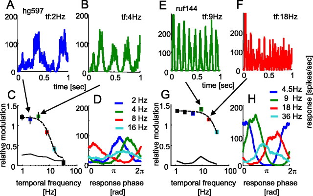
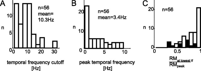
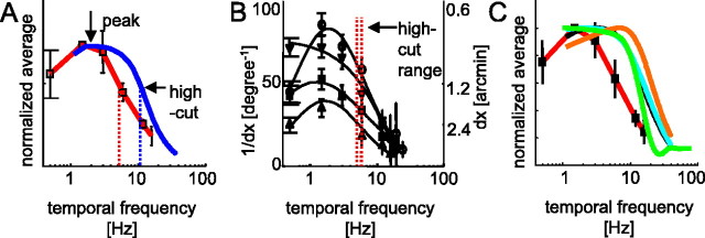
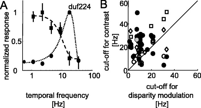
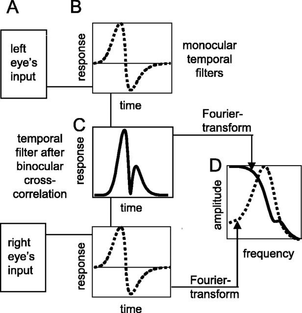
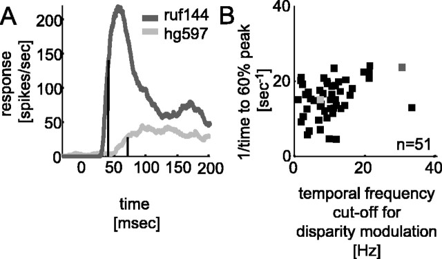
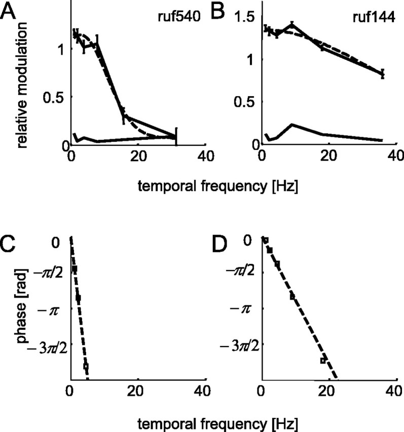
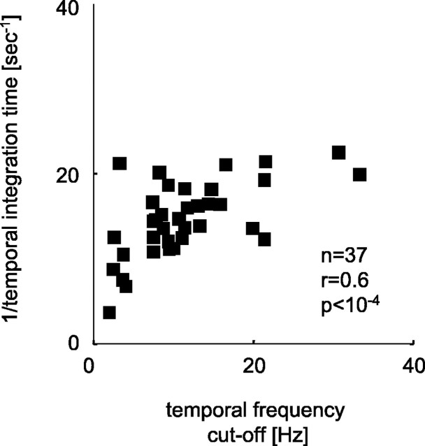
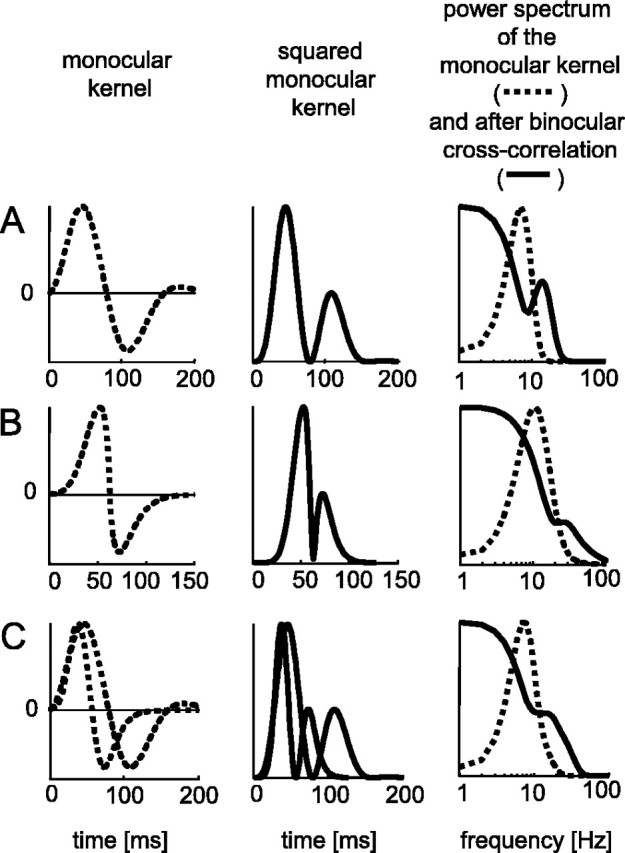
The human ability to detect modulation of binocular disparity over time is poor compared with detection of luminance modulation. We examined the physiological origin of this limitation by analyzing neuronal responses to temporal modulation of binocular disparity in striate cortex of awake monkeys. When neurons were presented with random-dot stereograms in which disparity varied sinusoidally over time, their responses modulated at the stimulus temporal frequency, with little change in mean firing rate. We calculated modulation amplitude as a function of temporal frequency and compared this with the psychophysical performance of four human observers. Neuronal and psychophysical functions showed similar peak frequencies (2 Hz) and comparable high-cut frequencies (10 and 5.5 Hz, respectively). Thus, V1 (primary visual cortex) neurons appear to limit psychophysical performance. The temporal resolution of the same neurons for contrast modulation was approximately 2.5 times greater, which parallels the superior psychophysical performance for contrast. There is a simple mathematical explanation for this difference: it results from calculating cross-correlation between temporally broadband monocular images that are bandpass filtered before measuring correlation. The limit on temporal resolution is a direct consequence of the binocular energy model that adds to the list of properties of human stereoscopic performance that are explained by this simple model of disparity encoding in V1: the same neurons can account for the performance of psychophysical tasks that result in either high (contrast) or low (disparity) temporal resolution. Because this principle holds whenever a broadband input is bandpass filtered before computing correlation, it may limit the resolution of other neuronal systems.

Figure 1.

Responses to disparity-modulating RDSs for two neurons (hg597, ruf144). A, B and E, F depict SDFs in response to disparity-modulating RDSs at different temporal frequencies (2 and 4 Hz for A and B; 9 and 18 Hz for E and F). D and H show cycle averages of the SDFs (2-16 and 4.5-36 Hz, respectively). The RM is plotted as a function of temporal frequency in C (cell hg597) and G (cell ruf144). Baseline RM (solid black line) is the modulation to a control stimulus (no disparity modulation) measured for the same temporal frequencies. The arrows point to the RM calculated for the data depicted in the respective panels A, B and E, F. RM plotted as a function of temporal frequency is fitted by Gaussian curves (dashed lines in C and G). High cutoff values were usually similar to that shown in C (8.1 Hz) but were significantly higher in a few neurons, as seen in G (35.3 Hz).

Figure 2.

Temporal frequency tuning of the cell population. A summarizes the high-frequency cutoff for 56 neurons. Mean value is 10.3 Hz. A frequency histogram of the peak temporal frequencies of the 56 neurons is shown in B (mean of 3.4 Hz). Most neurons had low peak temporal frequencies. The ratio of RM at the lowest temporal frequency over peak RM was used to estimate the extent of low-frequency attenuation (frequency histogram in C; n = 56). Filled bars correspond to cells with statistically significant low-frequency attenuation (n = 13; p < 0.05 by resampling).

Figure 3.

Comparing the neuronal population response with the psychophysical performance. A depicts the averaged Gaussian fits to the RM as a function of temporal frequency for the 56 neurons (blue solid line). The arrows indicate the high cutoff (10.5 Hz) and peak (2 Hz) for the averaged fits. Superimposed is the mean of the psychophysical performance (normalized for each subject by the value at 1.5 Hz) in response to disparity modulation for four human subjects (open squares, red solid line). Dotted lines indicate temporal frequency high-cut values. Psychophysical performance for each subject (n = 4) is shown in B. Sensitivity (1/disparity threshold; see Materials and Methods) is plotted as a function of temporal frequency. Mean high cutoff (two-thirds peak sensitivity) is 5.5 ± 0.4 Hz SD, and the range of the temporal frequency cutoffs between subjects is indicated by the dotted lines. In C, the influence of different pooling schemes is examined. The red curve shows the mean psychophysical performance and is identical to that in A. The orange curve depicts the average of the Gaussian fits for the 25% of the neurons (n = 14) with the highest temporal frequency cutoffs, the cyan of those 25% of the neurons (n = 14) with the highest RM values. For the black curve, the contribution of each fit (n = 56) is weighted according to the statistical reliability of RM (see Results) before being averaged. Cubic splines were also fit to all 56 neurons, and these fits were averaged (green curve).

Figure 4.

Temporal frequency cutoffs in response to contrast modulation are generally higher than in response to disparity modulation. A shows responses of one example neuron to disparity modulation (squares) and to drifting luminance gratings (circles). Axes show normalized responses [RM for disparity modulation, and firing rate (in spikes per second) for drifting gratings] as a function of temporal frequency (in Hertz). The temporal frequency high cuts are 7.5 and 26.4 Hz for disparity and contrast modulation, respectively. B, Filled symbols show the contrast temporal frequency cutoff values calculated from mean response rates; open symbols show cutoff values calculated from modulated responses. Note that, for counterphase-modulating stimuli, the ordinate refers to the frequency of the modulation in neuronal firing (i.e., twice the stimulus frequency because these are all complex cells). Temporal frequency cutoffs calculated from mean response rates to drifting luminance gratings were significantly higher than in response to disparity-modulating RDS (27 neurons; filled circles; neuron of A shown in gray): the geometric mean ratio is 2.3 (>1; p < 0.001). Ten cells showed modulation at the stimulus frequency in response to drifting gratings (f1 > f0, simple cells; open circles). For these cells, the cutoff frequency for the f1 component is plotted. For the remaining cells, the response modulation (f2 component) to counterphase-modulating stimuli, RDS (open diamonds; n = 11) or gratings (open squares; n = 8), was analyzed. For these 29 neurons, the geometric mean of the ratio in cutoff frequencies (all derived from modulated responses) is significantly higher than one (1.8; p < 0.001, by resampling).

Figure 5.

Schematic representation of the effect of bandpass filtering on the frequency response of the binocular cross-correlation. Input from the left and right eye (A) is passed through a temporal filter (B, dotted line). Appendix shows that the temporal kernel of the binocular cross-correlation (C, solid line) corresponds to the squared monocular kernel. D depicts the frequency response (bandpass) of the monocular kernel (dotted line) and of the binocular cross-correlation (solid line), which is low pass and has a lower cutoff frequency.

Figure 6.

Temporal frequency cutoff to disparity modulation and rise time at response onset. A shows averaged SDFs of the onset in response to disparity-modulating RDS. Solid lines mark the rise time to 60% peak. The neuron (ruf144) with the shorter rise time (42 ms; dark gray) has the higher temporal frequency cutoff (35.3 Hz). Neuron hg597 (light gray) has a rise time of 72 ms and a temporal frequency cutoff of 8.1 Hz. (The cells are the same for which the SDFs in Figure 1 are shown.) The scatter plot in B compares the temporal frequency cutoffs in response to disparity modulation with the reciprocal of the time to 60% peak at the response onset (n = 51; filled squares). The correlation is significant (r = 0.34; p < 0.01), as expected for the cross-correlation of bandpass-filtered images (see Results and Appendix).

Figure 7.

Phases of the neuronal responses. A and B depict two temporal frequency tuning functions in response to disparity modulation, plotting RM (ordinate) as a function of temporal frequency (abscissa). The temporal frequency cutoffs are 10.4 Hz (cell ruf540; A) and 35.3 Hz (cell ruf144; B). In C and D, the phase of the averaged SDF is plotted as a function of temporal frequency for the cells in A and B, respectively. The slope of the line relating phase and temporal frequency (dashed line) will be referred to as temporal integration time (206 and 44 ms for ruf540 and ruf144, respectively). Note the longer temporal integration time (steeper slope) for the neuron with the lower temporal frequency cutoff (ruf540; A, C).

Figure 8.

Temporal integration time and temporal frequency cutoff. Temporal frequency cutoffs were significantly correlated with the reciprocal temporal integration time (the slope of the line relating response phase and temporal frequency; see Fig. 7C,D) (n = 37; r = 0.59; p < 10^-4). The mean temporal integration time is 72 ± 23 ms SD.

Figure 9.

The intercept of the line relating phase of the response and temporal frequency with the ordinate. The intercept (in degrees) with the ordinate in the phase plots (Fig. 7C,D) is shown in the frequency histogram for 41 cells. Most values are close to 0° (mean of 10.6 ± 19.9° SD), suggesting that the neurons respond to the instantaneous disparity and not to motion in depth.

Figure 10.

The role of the shape of the bandpass filter for the binocular energy model. In the first and second columns, the monocular kernel (dotted line) and the squared monocular kernel (solid line) are shown, respectively. In column three, the frequency response of the squared monocular kernel (solid line) is superimposed on the monocular frequency response (dotted line). Row A, The kernel used resembles that known for the LGN. The frequency response for the squared kernel is low pass but has a second peak at double the peak frequency of the monocular kernel. Row B, the kernel is modified to have a steeper transition between the positive and negative lobes, such that the squared kernel is close to a single asymmetrical Gaussian function. The frequency response of the squared kernel therefore has only a small second peak and a cutoff at approximately half the cutoff frequency of the monocular kernel. Row C, Input from two subunits with slightly different temporal kernels (peak frequencies are 7 and 10 Hz, respectively) converge onto a binocular cell. The frequency response of the sum of the squared monocular kernels has only very small peaks at double the peak frequencies of the monocular kernel and a cutoff at approximately half the cutoff frequency of the sum of the monocular kernels.

References

1. Adelson EH, Bergen JR (1985) Spatiotemporal energy models for the perception of motion. J Opt Soc Am A 2: 284-299. - PubMed
1. Albrecht DG (1995) Visual cortex neurons in monkey and cat: effect of contrast on the spatial and temporal phase transfer functions. Vis Neurosci 12: 1191-1210. - PubMed
1. Anzai A, Ohzawa I, Freeman RD (1999) Neural mechanisms for processing binocular information. II. Complex cells. J Neurophysiol 82: 909-924. - PubMed
1. Banks MS, Gepshtein S, Landy MS (2004) Why is spatial stereoresolution so low? J Neurosci 24: 2077-2089. - PMC - PubMed
1. Barlow HB, Blakemore C, Pettigrew JD (1967) The neural mechanism of binocular depth discrimination. J Physiol (Lond) 193: 327-342. - PMC - PubMed
Publication types
LinkOut - more resources