Do we know what the early visual system does?

Abstract

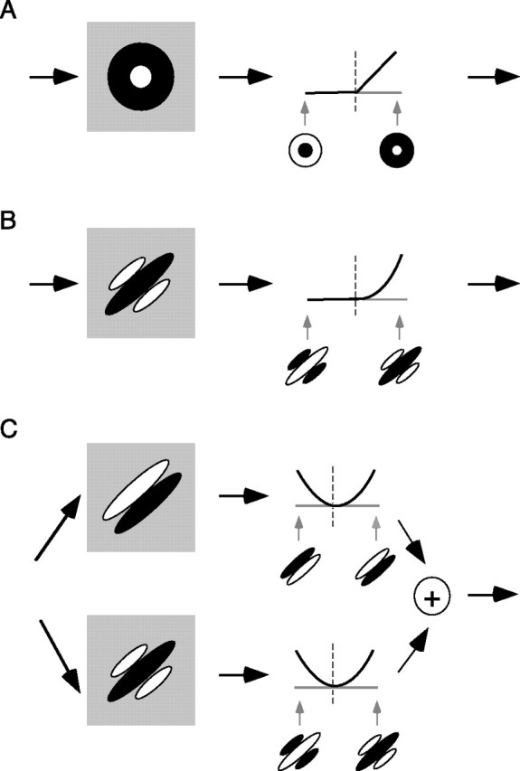
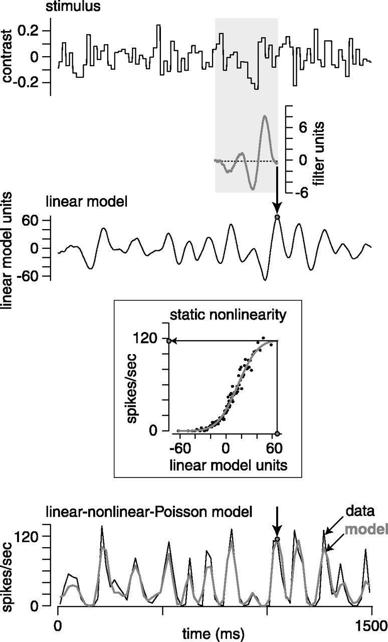
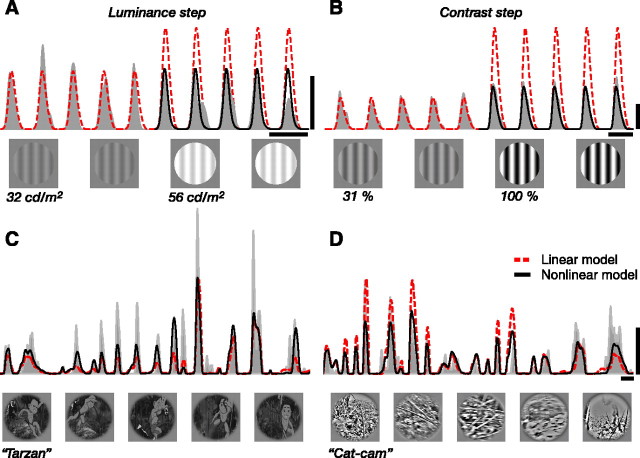
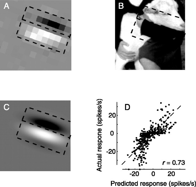
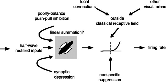
We can claim that we know what the visual system does once we can predict neural responses to arbitrary stimuli, including those seen in nature. In the early visual system, models based on one or more linear receptive fields hold promise to achieve this goal as long as the models include nonlinear mechanisms that control responsiveness, based on stimulus context and history, and take into account the nonlinearity of spike generation. These linear and nonlinear mechanisms might be the only essential determinants of the response, or alternatively, there may be additional fundamental determinants yet to be identified. Research is progressing with the goals of defining a single "standard model" for each stage of the visual pathway and testing the predictive power of these models on the responses to movies of natural scenes. These predictive models represent, at a given stage of the visual pathway, a compact description of visual computation. They would be an invaluable guide for understanding the underlying biophysical and anatomical mechanisms and relating neural responses to visual perception.

Figure 1.

Basic models of neurons involved in early visual processing. In all models, the response of a neuron is described by passing an image through one or more linear filters (by taking the dot product or projection of an image and a filter). The outputs of the linear filters are passed through an instantaneous nonlinear function, plotted here as firing rate on the ordinate and filter output on the abscissa. A, Simple model of a retinal ganglion cell or of an LGN relay neuron. The model includes a linear filter (receptive field) with a center-surround organization and a half-wave rectifying nonlinearity. Images that resemble the filter produce large firing rate responses, whereas images that resemble the inverse of the filter or have no similarity with the filter produce no response. B, Model of a V1 simple cell as a filter elongated along one axis and a half-wave squaring nonlinearity. As in A, only images that resemble the filter produce high firing rate responses. C, The energy model of a V1 complex cell. The model includes two phase-shifted linear filters whose outputs are squared before they are summed. In this model, both images that resemble the filters and their inverses produce high firing rates.

Figure 2.

The LNP model of the spike response in a retinal ganglion cell. A model of an ON Y-type ganglion cell was generated from 100 s of response to a white-noise stimulus, contrast was 0.1, extra cellular recording in in vitro guinea pig retina; methods as described by Zaghloul et al. (2005). The model generates a linear filter (weighting function) and a static nonlinearity (Chichilnisky, 2001). To predict the response to a novel dataset, the stimulus is passed through the filter to generate the linear model of the response. The filter is shown at a time when it closely matched the stimulus (gray box), and so the linear model response is large (+63 in linear model units; gray circle). The linear model is translated to a spike rate using a static nonlinearity that works like a “lookup table” (shown in box). The point in the linear model at +63 is translated to a spike rate of 117 spikes/s. The bottom trace shows the spike rate (black line) to 1.5 s of the novel stimulus (of 2.7 s total). The test stimulus was repeated 20 times, and the data were averaged and binned (bin, 20 ms). The gray line shows the output of the LNP model (bin, 20 ms). The gray circle shows the LNP model value at 117 spikes/s at the same time shown above for the linear model. The r² between the data and model was 0.81.

Figure 3.

Predicting responses of LGN neurons to complex video sequences. A, Firing rate responses of an LGN neuron to a drifting grating whose mean luminance is suddenly increased from 32 to 56 cd/m² (while contrast is kept constant). Red dashed traces indicate the prediction of the linear receptive field fitted to the response before the luminance step, and black solid traces indicate the average response after the step. B, Same, for a stimulus whose contrast suddenly steps from 31 to 100% (while mean luminance is kept constant). C, Responses of an LGN neuron to a sequence from Walt Disney's Tarzan. Red dashed traces indicate the prediction of the linear receptive field alone (measured at optimal luminance and contrast). Black solid traces indicate prediction of a nonlinear model. In the nonlinear model, the gain and integration time of the receptive field are regulated by luminance gain control and contrast gain control. D, Same, for responses to a Cat-cam movie (Kayser et al., 2003; Betsch et al., 2004). In all panels, calibration is 100 ms and 100 spikes/s, and gray histograms are firing rates obtained by convolving the spike trains with a Gaussian window of width 5 ms (SD). A and B are modified from Mante et al. (2005b). C and D are modified from Mante (2005).

Figure 4.

Predicting responses of V1 simple cells to complex images. A, The receptive field of a ferret simple cell (see Fig. 1 B). The dashed lines outline the field for comparison in B and C. B, The digitized photograph that evoked the largest OFF response in this simple cell. C, A Gabor patch that approximately matches the disposition of the actual receptive field in A. D, The ordinate plots the actual responses of the simple cell to 500 different photographs (average of 10 presentations each, measured in 100 ms bins). Positive values are ON responses: spikes generated during the 100 ms presentation. Negative values are OFF responses: spikes generated on removal of the photograph. The abscissa shows the responses predicted on a totally linear model, which includes solely the receptive field shown inC and not the nonlinearity of the output (see Fig. 1 B).

Figure 5.

Toward a complete model of V1 simple cells. A popular conception of simple-cell response behavior involves a first stage that shows strictly linear spatiotemporal summation, and a subsequent stage may be subject to a variety of nonlinear phenomena, which do not impinge on the fundamental linearity of the first stage (see Fig. 1 B). This schematic shows a revision of this convenient model, which includes a number of nonlinear mechanisms. Some of these mechanisms (those depicted as affecting the output nonlinearity) spare the fundamental linearity of summation. The remaining ones, however, cause nonlinear summation, which differs only in degree from the obvious nonlinear behavior of complex cells.

Figure 6.

Models of V1 complex cells recovered from a covariance analysis. A, Experimental protocol. Top, A segment of the natural image ensemble; white box indicates area shown in experiments. Bottom, Spike train. Spike-triggered ensemble was generated by collecting the image preceding each spike by a single frame (42 ms). B, Two significant eigenvectors of a complex cell. Scale bar, 2°. Solid line, Spatial profiles of each eigenvector along the axis perpendicular to the preferred orientation. Dashed line, Gabor fit. The Gabor fits of the two eigenvectors had a phase difference of 85°. C, Contrast-response functions of the two eigenvectors. Average firing rate is plotted against the contrast of each eigenvector shown in B. Error bar indicates ±SEM. Dashed lines, Fits of the data with the function r(x) =β x^γ + r₀, where r is the firing rate, x is contrast, and β, γ, and r₀ are free parameters. D, E, Prediction of cortical responses to natural images. Correlation coefficients between the predicted and measured responses based on the eigenvectors were plotted again those based on the linear receptive field (D) and against the estimated upper bound (E). Each symbol represents one complex cell.

Figure 7.

Spatial receptive fields of four V1 neurons estimated using dynamic grating sequences (top row) and dynamic sequences of natural images (bottom row). The spatial receptive field describes selectivity in terms of a joint orientation-spatial frequency tuning surface. Each point in a spatial receptive field map describes the relative response to a stimulus of a particular orientation and spatial frequency (angle about the origin and distance from the origin, respectively; see legend at right). Red indicates orient at ions and spatial frequencies that tended to increase responses; blue indicates decreased responses. Both gratings and natural images yield spatial receptive fields in which excitatory tuning is centered around a small range of spatial frequencies and orientations. Inhibitory tuning tends to be more diffuse, and its structure depends on the stimulus.

References

1. Adelson EH, Bergen JR (1985) Spatiotemporal energy models for the perception of motion. J Opt Soc Am A 2: 284-299. - PubMed
1. Albrecht DG, Geisler WS (1991) Motion selectivity and the contrast-response function of simple cells in the visual cortex. Vis Neurosci 7: 531-546. - PubMed
1. Albrecht DG, Hamilton DB (1982) Striate cortex of monkey and cat: contrast response function. J Neurophysiol 48: 217-237. - PubMed
1. Albright TD, Stoner GR (2002) Contextual influences on visual processing. Annu Rev Neurosci 25: 339-379. - PubMed
1. Andrews BW, Pollen DA (1979) Relationship between spatial frequency selectivity and receptive field profile of simple cells. J Physiol (Lond) 287: 163-176. - PMC - PubMed
LinkOut - more resources