Prediction and decoding of retinal ganglion cell responses with a probabilistic spiking model

Abstract

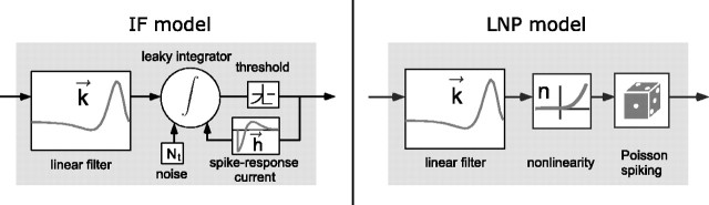
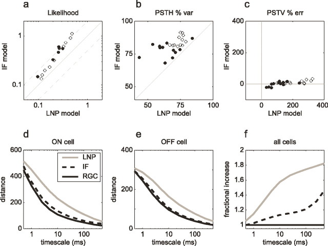
Sensory encoding in spiking neurons depends on both the integration of sensory inputs and the intrinsic dynamics and variability of spike generation. We show that the stimulus selectivity, reliability, and timing precision of primate retinal ganglion cell (RGC) light responses can be reproduced accurately with a simple model consisting of a leaky integrate-and-fire spike generator driven by a linearly filtered stimulus, a postspike current, and a Gaussian noise current. We fit model parameters for individual RGCs by maximizing the likelihood of observed spike responses to a stochastic visual stimulus. Although compact, the fitted model predicts the detailed time structure of responses to novel stimuli, accurately capturing the interaction between the spiking history and sensory stimulus selectivity. The model also accounts for the variability in responses to repeated stimuli, even when fit to data from a single (nonrepeating) stimulus sequence. Finally, the model can be used to derive an explicit, maximum-likelihood decoding rule for neural spike trains, thus providing a tool for assessing the limitations that spiking variability imposes on sensory performance.

Figure 1.

Schematic diagrams of the generalized IF model (left) and the standard LNP model (right).

Figure 2.

Parameters obtained from fits to RGC data for the IF model (a-c) and the LNP model (d, e). a, Filters and spike-response currents obtained for five ON cells in one retina. b, Corresponding filters for four OFF cells. c, Histograms of model scalar parameters and for all 24 cells in three retinas. d, Comparison of linear filters for the IF model (gray) and LNP model (black) for one ON cell (top) and one OFF cell (bottom). e, Measured LNP point nonlinearities for converting filter output to instantaneous spike rate.

Figure 3.

Responses of an ON cell to a repeated stimulus. a, Recorded responses to repeated stimulus (top), simulated LNP model (middle), and IF model (bottom) spike trains. Each row corresponds to the response during a single stimulus repeat; 167 repeats are shown. b, PSTH, or mean spike rate, for the RGC, LNP model, and IF model. For this cell, the IF model accounts for 91% of the variance of the PSTH, where as the LNP model accounts for 75%. c, Spike count variance computed in a sliding 10 ms window. d, Magnified sections of rasters, with rows sorted in order of first spike time within the window. The four sections shown are indicated by blue brackets in a.

Figure 4.

Responses of an OFF cell to a repeated stimulus. Details are identical to those of Figure 3.

Figure 5.

Performance comparison across cells. Open and filled circles represent ON and OFF cells, respectively. a, Likelihood per spike of novel RGC responses under the fitted IF model and LNP model. The value plotted is the geometric mean of the likelihood of over all spikes under each model. Gray dashed lines represent a factor of 2 above and below identity. Data from 24 cells (3 retinas) are shown. b, Percentage variance (var) in the PSTH accounted for by both models for each cell. Points above the diagonal represent superior performance by the IF model. c, Percentage error (err) in the peristimulus time variance for the IF and LNP models across cells. d, Average pair-wise distance between spike trains as a function of time scale of analysis (see Results). Black trace, Median distance between responses of an ON RGC to repeated presentations of the same stimulus; dashed trace, median distance between IF model response and data; gray trace, median distance between LNP model response and data. e, Same as d for an OFF RGC. f, Fractional increase in spike-time distance for the IF and LNP models averaged over all cells. Dashed curve, Ratio of IF model distance to the average pair-wise distance between RGC responses, normalized by the number of spikes from each cell and averaged across cells; gray curve, same for LNP model.

Figure 6.

IF model prediction of responses to brief flashes. a, b, ON cell responses and IF model predictions. c, d, OFF cell responses and IF model predictions. The flash stimuli (shown above each raster) consisted of a gray screen followed by a brief (25 ms) flash. Flash contrasts were +12, +24, +48, and +96% (pos. flashes; a, c) and -12, -24, -48, and -96% (neg. flashes; b, d). Below each stimulus is a raster showing 25 responses of the RGC (black), below which is a raster showing 25 simulated responses of the IF model (red). Below each pair of rasters is a plot of the PSTH of the RGC and IF model on the same axes. For these two cells, the IF model accounted for 76 and 90% of the PSTH variance for the ON and OFF cells, respectively.

Figure 7.

Precision of firing onset times. a, Two hundred millisecond portion of stimulus and a response raster showing two periods of firing onset. Below are histograms of the time of the first spike in each event. SDs, 1.3 ms (left); 4.7 ms (right). b, Simulated voltage response from the fitted IF model with noise set to zero. Tangent at time of firing onset is shown in gray. c, Precision of first spike times (inverse of SD) as a function of the mean current at the time of the first spike over 70 isolated firing onsets. Correlation coefficient, 0.89. d, Correlation coefficient (corr coeff) between precision and IF model current prediction as a function of the inverse of the average SD of the first spike time. Open circles denote ON cells, and filled circles denote OFF cells.

Figure 8.

Generalized analysis of timing precision. a, RGC response raster sorted in order of first spike time. Below is a histogram of first spike (gray) and second spike (black) in the event, illustrating higher precision in the time of the second spike than the first. b, Sorted RGC response raster, with histograms below showing the distribution of the first (gray) and last (black) spikes in this event. Precision of the last spike is higher than the first. c-e, Use of the IF model formalism to analyze RGC spike timing precision and reliability. c, One hundred seventy millisecond stimulus fragment and corresponding RGC spike response during one trial. d, Probability distribution over subthreshold voltage for a central interspike interval on a single trial. The likelihood of the next spike time (below) is given by the probability mass crossing the threshold at each moment in time. Note that the probability distribution of the next spike time is bimodal. e, Raster of repeated RGC responses to this stimulus fragment, with rows sorted in order of first spike time. Below is the probability density of the next spike, averaged across 25 trials. Black trace, Model prediction; gray bars, actual distribution.

Figure 9.

Decoding responses using model-derived likelihoods. a, Two stimulus (Stim) fragments and corresponding fragments of the RGC response (Resp) raster. Gray boxes highlight a 50 ms interval of the first row of each response raster. A 2AFC discrimination task was performed on these response fragments, in which the task was to determine which stimulus gave rise to each response. The IF and LNP models were used to compute the likelihood of these responses given the “correct” and “incorrect” pairing of stimuli and responses, and the pairing with the higher likelihood was selected. This discrimination procedure was applied to each row of the response raster and used to obtain the percentage correct for the discrimination performance of each model. b, Discrimination performance of the IF and LNP models. Each point corresponds to the percentage correct of a 2AFC discrimination task using two randomly selected 50 ms windows of the response. Although both models obtain perfect performance (100%) for a majority of such randomly selected response windows, the scatter of points above the diagonal shows that when discrimination performance is imperfect, the IF model is far better at decoding the neural spike responses.

References

1. Aguera y Arcas B, Fairhall AL (2003) What causes a neuron to spike? Neural Comput 15: 1789-1807. - PubMed
1. Baccus SA, Meister M (2002) Fast and slow contrast adaptation in retinal circuitry. Neuron 36: 909-919. - PubMed
1. Banerjee A (2001) On the phase-space dynamics of systems of spiking neurons, ii: formal analysis. Neural Comput 13: 195-225. - PubMed
1. Benardete EA, Kaplan E, Knight BW (1992) Contrast gain control in the primate retina: P cells are not X-like, some M cells are. Vis Neurosci 8: 483-486. - PubMed
1. Berry M, Meister M (1998) Refractoriness and neural precision. J Neurosci 18: 2200-2211. - PMC - PubMed
Publication types