Attention modulates the responses of simple cells in monkey primary visual cortex

Abstract

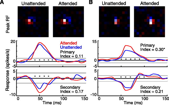
Spatial attention has long been postulated to act as a spotlight that increases the salience of visual stimuli at the attended location. We examined the effects of attention on the receptive fields of simple cells in primary visual cortex (V1) by training macaque monkeys to perform a task with two modes. In the attended mode, the stimuli relevant to the animal's task overlay the receptive field of the neuron being recorded. In the unattended mode, the animal was cued to attend to stimuli outside the receptive field of that neuron. The relevant stimulus, a colored pixel, was briefly presented within a white-noise stimulus, a flickering grid of black and white pixels. The receptive fields of the neurons were mapped by correlating spikes with the white-noise stimulus in both attended and unattended modes. We found that attention could cause significant modulation of the visually evoked response despite an absence of significant effects on the overall firing rates. On further examination of the relationship between the strength of the visual stimulation and the firing rate, we found that attention appears to cause multiplicative scaling of the visually evoked responses of simple cells, demonstrating that attention reaches back to the initial stages of visual cortical processing.

Figure 1.

Stimulus configuration and behavioral protocol. The animal fixated on the central spot and had previously been cued to direct his attention to one of the two stimulus grids. The blue dashed circle represents the receptive field of the recorded neuron and was not present on the screen. Trials in which the animal's attention was directed to the grid overlying the receptive field were defined as attended, whereas those trials in which his attention was directed to the other grid were defined as unattended. A small colored patch (in this example, follow the dashed blue arrow to a red square in the top left stimulus grid) was visible for 250-350 ms, during which time all of the other pixels in the stimulus continued to change luminance randomly. If the animal's attention had been cued to the grid on the top left, the correct response would be a saccade to the red target, illustrated by the solid blue arrow. If the animal's attention had been directed to the stimulus grid on the bottom right (no colored patch shown in this example), the correct response would have been to maintain fixation. Such catch trials ended after a random interval ranging from 260 to 3300 ms.

Figure 2.

A, The spatiotemporal receptive-field map of a single neuron in the unattended mode (top) and attended mode (bottom). Blue indicates regions in which black pixels tended to precede spikes (off responses, negative values), and red indicates regions in which white pixels preceded spikes (on responses, positive values). Brighter colors indicate more responsive areas of the receptive field. Intersections in the grid lines correspond to centers of the stimulus pixels. Response values were interpolated between pixels. The unattended maps were generated from 2473 spikes and 5260 frames over 108 correct trials, and the attended maps were generated from 2438 spikes and 5160 frames over 108 correct trials. B, The spatial receptive-field (RF) maps were extracted from the spatiotemporal maps by averaging the time frames near the peak response and selecting pixels meeting threshold levels and contiguous with other strong pixels (see Materials and Methods). This was done independently for the primary (column 2) and secondary (column 3) sub fields and for both behavioral modes (red and white pixels). However, only those pixels that overlapped in the two behavioral modes were included in the comparison (white pixels). C, The time courses of the responses for the receptive-field subfields, summed over all white pixels defined in B. Attended modes are shown in red, and unattended modes are in blue. The gray lines show ±3 SDs of the noise (pixel variability times the square root of the number of pixels composing the spatial receptive-field subregion) in the response. The asterisks along the x-axis indicate those time bins in which the responses were >3 SDs of the noise for both the attended and unattended modes and were summed to determine the total visual responses for each mode and each subregion.

Figure 3.

Spatiotemporal receptive-field maps (unattended, left; attended, right) and time courses of the responses of the receptive-field (RF) subfields (primary, top; secondary, bottom) for two single neurons that showed modest effects of attention. For the neuron in A, the unattended maps were generated from 1370 spikes and 4573 frames over 108 correct trials, and the attended maps were generated from 1559 spikes and 4991 frames over 108 correct trials. For the neuron in B, the unattended maps were generated from 2170 spikes and 5924 frames over 144 correct trials, and the attended maps were generated from 2539 spikes and 5526 frames over 144 correct trials.

Figure 4.

Histograms of the attentional modulation index for the primary subfield (A) and the secondary subfield (B). The attentional modulation index was defined as the attended response minus the unattended response divided by their mean. Cells shown in black had individually statistically significant effects of attention.

Figure 5.

Spatial and temporal receptive fields calculated with and without correction for eye position. Two different neurons are shown in A and B. For each, the spatial receptive fields (RF) in the unattended, attended, and the pixels chosen for analysis of the primary subfield are shown on the left. The time course of the responses in those pixels is shown on the right. The top row for each neuron are the original (uncorrected) maps, and the bottom row are the maps after adjusting for the actual eye position relative to the white-noise stimulus, at a resolution of a quarter of each pixel, at the time of the spikes. Both neurons had individually significant effects of attention both with and without eye correction. Neuron A is the same neuron shown in Figure 2. The attentional index value for each condition is displayed on the top left of the time response function.

Figure 6.

A, Histogram of the attentional modulation index of the primary sub field (as in Fig. 4), calculated with the correction for eye position. The 13 cells shown in black had individually statistically significant effects of attention. B, The attentional index for the primary subfield without the correction for eye position is plotted against the attentional index with the correction for eye position. The diagonal x = y is plotted as well. Filled symbols indicate cells with significant effects: filled circles indicate effects only without eye correction (3 cells); filled squares indicate effects only after eye correction (3 cells); and filled triangles indicate effects in both cases (10 cells).

Figure 7.

A, The time course of the responses for the 12 neurons with individually significant positive effects of attention were constructed by normalizing each cell to its peak response in the unattended mode and then shifting each function so that the peak responses of each neuron were aligned in time. The attended mode is in black, the unattended mode in dark gray, and their difference is shown with a dashed black line. B, The attentional index for the peak of the primary subfield is plotted against the attentional index for the peak of the antagonistic subfield. The diagonal x = y is plotted as well. Filled symbols indicate cells with significant differences between the attentional states: filled circles indicate an effect on the primary subfield only (10 cells); filled squares indicate an effect on the secondary subfield only (3 cells); and filled triangles indicate the cells with effects on both subfields (3 cells).

Figure 8.

A, Histograms of the attentional modulation index for the overall firing rate in response to the stimulus. The attentional modulation index was defined as the spike rate in the attended mode minus the spike rate in the unattended mode divided by their mean. No cells showed individually significant changes in spike rate. B, The attentional index for the primary subfield is plotted against the attentional index for the overall spike rate in response to all stimuli. The 13 cells with significant effects on the primary subfield are shown as filled circles.

Figure 9.

Computation of the two-stage model: a linear filter followed by a nonlinear output function. First row, Schematic representation of four successive stimulus frames, with additional frames indicated by black dots. Second row, The receptive field of a single neuron is convolved with the stimulus sequence to provide a single numerical value representing the result of the linear first stage (the “linear input”). Third row, A portion of the calculated output of the linear first stage, arbitrarily scaled from -1 to 1; the x-axis is time and covers 40 different stimulus frames at 23.5 ms/frame. The open circle is the value derived from the stimuli illustrated in the first row; the neighboring black dots indicate the values for the adjacent stimulus frame sequences. Fourth row, A simple form of output nonlinearity: a rectifier that converts all negative inputs to zero and linearly scales positive inputs. Fifth row, Green, The predicted firing rate, derived by passing the result of the linear stage through the output function. The lines shown in red, on the bottom axis, are the actual spikes of the neuron, which varied from zero to three spikes per frame within this specific sequence and up to five spikes per frame overall. The neuron fired more spikes when the predicted firing rate function is high and few or no spikes when the predicted firing rate is low.

Figure 10.

The output functions for a single neuron (A) and for the 15 cells with strongest attentional modulation (B). The output functions (black, attended mode; gray, unattended mode) represent the firing rate (y-axis) averaged over all frames for which the linear first stage took on a particular range of values (x-axis). In A, the dots indicate the SEM for each bin. The dashed line is the average undriven response of the neuron during the fixation period (no stimuli in receptive field). In B, the linear inputs from each neuron were aligned on the maximum value of its linear first stage, and the axis was fixed from -1.0 to 1.0. The responses of each neuron were normalized to the peak response in the unattended mode before averaging across the neurons. The error bars indicate the SE in the normalized bins across neurons. InC, the normalized attended response is plotted against the normalized unattended response for the 15 cells with the strongest attentional modulation (filled circles). The black line shown is the linear regression of the attended responses on the unattended responses (y = 1.24x-0.02; r² = 0.994). The gray line (y = x) is the expected result if there was no effect of attention. The SE bars are plotted at each point, for both the attended and unattended response values. The dashed black lines show ±1 SEM of the normalized undriven activity. Renormalized data from area V4 from McAdams and Maunsell (1999) has been plotted using open diamonds for the response values and dashed gray lines to indicate the undriven activity in that study (see Results). In D, we show the population average of the distributions of the number of times bins (circles) and total spikes (lines) occurred for each value of the linear input for the same 15 cells as in B and C (black, attended; gray, unattended). There were many more time bins, and subsequently more total spikes, for linear input values near zero; the most effective stimuli occurred only rarely and evoked relatively few total spikes.

References

1. Brefczynski JA, DeYoe EA (1999) A physiological correlate of the “spotlight” of visual attention. Nat Neurosci 2: 370-374. - PubMed
1. Carandini M, Ferster D (2000) Membrane potential and firing rate in cat primary visual cortex. J Neurosci 20: 470-484. - PMC - PubMed
1. Cave KR, Bichot NP (1999) Visuospatial attention: beyond a spotlight model. Psychon Bull Rev 6: 204-223. - PubMed
1. Chichilnisky EJ (2001) A simple white noise analysis of neuronal light responses. Network 12: 199-213. - PubMed
1. Chung S, Ferster D (1998) Strength and orientation tuning of the thalamic input to simple cells revealed by electrically evoked cortical suppression. Neuron 20: 1177-1189. - PubMed
Publication types