Reduction of false positives by internal features for polyp detection in CT-based virtual colonoscopy

Abstract

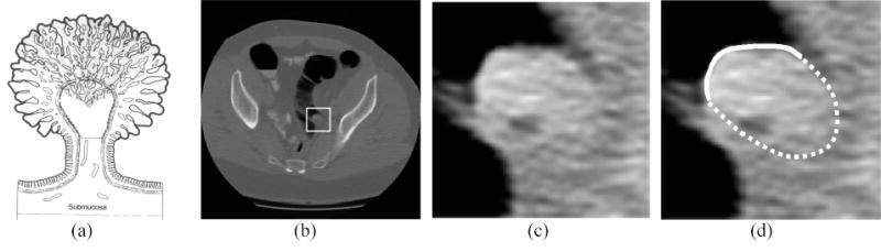
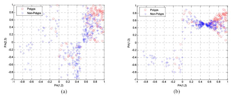
In this paper, we present a computer-aided detection (CAD) method to extract and use internal features to reduce false positive (FP) rate generated by surface-based measures on the inner colon wall in computed tomographic (CT) colonography. Firstly, a new shape description global curvature, which can provide an overall shape description of the colon wall, is introduced to improve the detection of suspicious patches on the colon wall whose geometrical features are similar to that of the colonic polyps. By a ray-driven edge finder, the volume of each detected patch is extracted as a fitted ellipsoid model. Within the ellipsoid model, CT image density distribution is analyzed. Three types of (geometrical, morphological, and textural) internal features are extracted and applied to eliminate the FPs from the detected patches. The presented CAD method was tested by a total of 153 patient datasets in which 45 patients were found with 61 polyps of sizes 4-30 mm by optical colonoscopy. For a 100% detection sensitivity (on polyps), the presented CAD method had an average FPs of 2.68 per patient dataset and eliminated 93.1% of FPs generated by the surface-based measures. The presented CAD method was also evaluated by different polyp sizes. For polyp sizes of 10-30 mm, the method achieved mean number of FPs per dataset of 2.0 with 100% sensitivity. For polyp sizes of 4-10 mm, the method achieved 3.44 FP per dataset with 100% sensitivity.

Figure 1

Illustration of two different kernel functions – Uniform kernel (left) and Gaussian kernel (right).

Figure 2

(a) Illustration of a colonic polyp which is fully inside the lumen and has a typical elliptical shape. (b) In a CT image, the geometrical feature of a polyp (indicated by the white rectangle) becomes blurred. (c) The zoomed display of the polyp which shows some kinds of “elliptical” shape for both the detected portion inside the lumen and the inner portion inside the wall. (d) In a CT image, a polyp only shows part of its whole border inside the lumen. The solid curve indicates the outer border in the lumen; the dashed curve indicates the inner border behind the surface which can not be detected by the shape analysis on the surface directly.

Figure 3

(a) 2D illustration of three rays emitted from a given voxel (indicated by the cross) in a candidate. (b) The CT density profile along Ray_grad, i.e., the middle arrow toward the bottom right in (a). (c) The step-like profile after the Harr wavelet transformation and filtering. (d) The coding sequence of the step-like profile. The above is the initial coding sequence. After merging some small parts, we get the final coding as shown in the bottom. (e) Some special variance pattern can be detected using the coding sequence and the exact position is identified by the first- and second-order derivatives of the original profile. The detected point is indicated by the arrow. Meanwhile, we define a search range (indicated by the dotted vertical line) to reduce the possibility of finding a wrong edge. (f) The detected three new border points (the crosses) along the three rays, respectively. Among them, two are the outer border points, and one is the inner border point.

Figure 4

Illustration of Harr wavelet transformation in the edge detector.

Figure 5

(a-1) A polyp (6 mm in diameter) in a CT image. The solid curve indicates all the outer border points which are grouped into the initial candidate. (a-2) The ellipsoid (dashed line) constructed using only the outer border points in the left image. This ellipsoid may only cover a portion of the polyp. (a-3) The ellipsoid generated using both the outer and the inner border points. All the inner border pointes are detected using the ray-driven edge finder. (b-1) Another polyp candidate (10 mm in diameter) with irregular surface. Its outer border points are grouped into two different candidates. (b-2) Two different ellipsoids are generated. Either of them covers the whole polyp volume. (b-3) A new ellipsoid generated is generated by merging the two candidates. (c) Another example for a candidate of 7 mm in diameter and its corresponding ellipsoid. (d) Another candidate of 15 mm in diameter which covers only a small section of the whole border of the polyp, and its ellipsoid generated from the small solid curve using the ray-driven edge finder. (e) An example of two polyp-like colon folds which can not be eliminated by the shape analysis and become polyp candidates, resulting in two ellipsoids. However, due to the lack of inner border information, the upper ellipsoid is spindly. Although the lower ellipsoid shows a similar shape as a true polyp, it has much less inner border information than a true polyp has and, therefore, is likely to be eliminated by the texture information derived from the ellipsoid as discussed in the next section.

Figure 6

(a) Illustration and definition of the enlarged and shrunk borders for an eROI. (b) The three borders in a CT image. The solid line represents the original border of the eROI; and the two dashed lines represent the shrunk border and the enlarged border of the eROI respectively.

Figure 7

The 2D/3D plots of the triple-element vectors of voxels from polyps and non-polyps (or FPs). All voxels are selected by the computer randomly. Pictures (a)–(c) show the 2D plots of the triple-element vectors. Picture (d) shows the 3D plot. The triple-element vectors of polyp voxels show a convergence toward the top right corner (by the circles).

Figure 7

The 2D/3D plots of the triple-element vectors of voxels from polyps and non-polyps (or FPs). All voxels are selected by the computer randomly. Pictures (a)–(c) show the 2D plots of the triple-element vectors. Picture (d) shows the 3D plot. The triple-element vectors of polyp voxels show a convergence toward the top right corner (by the circles).

Figure 8

Illustration of the mapping procedure of octsphere parameterization. Picture (a) shows the parameterization of the ellipsoid surface or border. The whole surface is divided into many triangular patches. In picture (b), a CT density profile is drawn, for each patch, along the gradient ray emitted from its central point. The search range is defined by the intersection points of the ray with the enlarged and shrunk borders. If there exists a border in the given search range, this patch is marked (or colored by the red in picture (c)). Picture (d) shows the mapped image. The gray patches indicate all marked patches, and the black (darker) patches are the un-marked patches. Picture (e) shows a patch pair.

Figure 9

Illustrations of a transformation function (left) and a two-level classifier for the final polyp identification (right).

Figure 10

The FROC curve of the presented CAD scheme for the 153 patient datasets. (a) The FROC curves of the presented CAD scheme for different polyp sizes. (b) The FROC curves for the CAD scheme with different groups of the internal features from all datasets.

Figure 11

The ROC curves resulted from polyp detection using different curvatures. Notation “Uniform [x] mm” indicates the result of the global curvature with uniform kernel function and a half curve length of x mm; and “Gaussian-[x]” is the result of the global curvature with Gaussian kernel function and an alpha value of “x” mm. Notation “+Uniform” shows the result of combination of the local and global curvatures. (a) The ROC curves using the local and global curvatures, respectively. (b) The ROC curves using the combination of the local and global curvatures.

References

1. “Cancer Facts & Figures 2004”, American Cancer Society Annual Report, 2004.
1. O’Brien M, Winawer S, Zauber A, Gottlieb L, Sternberg S, Diaz B, Dickersin G, Ewing S, Geller S, Kasimian D. “The national polyp study: patient and polyp characteristics associated with high-grade dysplasia in colorectal adenomas”. Gastroenterology. 1990;98(2):371–379. - PubMed
1. Coin C, Wollett F, Coin J, Rowland M, Deramos R, Dandrea R. “Computerized radiology of the colon: A potential screening technique”. Comput Radiology. 1983;7(1):215–221. - PubMed
1. Vining D, Gelfand D, Bechtold R, Scharling E, Grishaw E, Shifrin R. “Technical feasibility of colon imaging with helical CT and virtual reality”. Annual Meeting of American Roentgen Ray Society, New Orleans. 1994:104.
1. W. Lorensen, F. Jolesz, and R. Kikinis, “The exploration of cross-sectional data with a virtual endoscope”, in R. Satava and K. Morgan (eds), Interactive Tech and New Med Paradigm for Health Care, IOS Press, Washington, DC, pp. 221–230, 1995.
Publication types