Visual clutter causes high-magnitude errors

Abstract

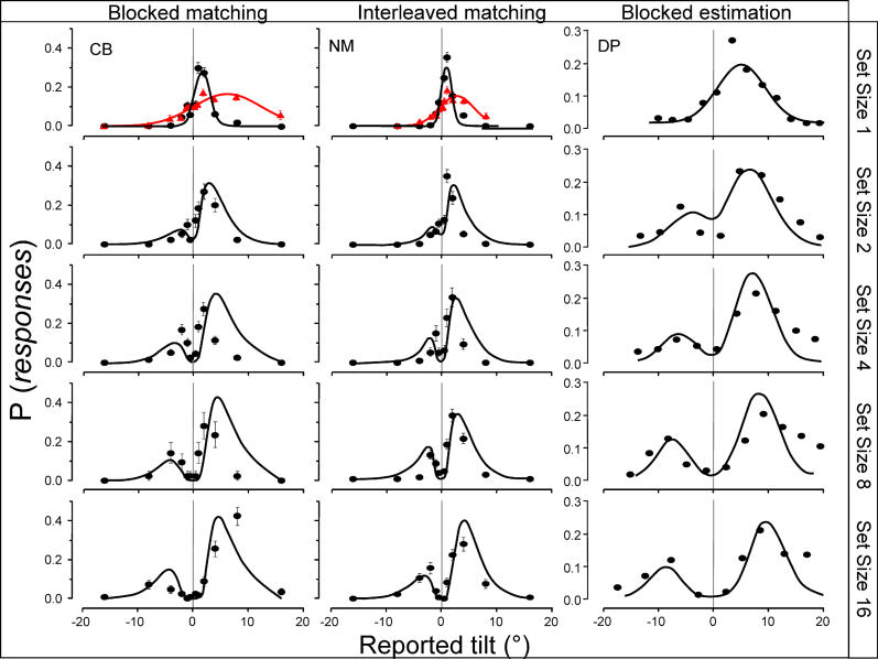
Perceptual decisions are often made in cluttered environments, where a target may be confounded with competing "distractor" stimuli. Although many studies and theoretical treatments have highlighted the effect of distractors on performance, it remains unclear how they affect the quality of perceptual decisions. Here we show that perceptual clutter leads not only to an increase in judgment errors, but also to an increase in perceived signal strength and decision confidence on erroneous trials. Observers reported simultaneously the direction and magnitude of the tilt of a target grating presented either alone, or together with vertical distractor stimuli. When presented in isolation, observers perceived isolated targets as only slightly tilted on error trials, and had little confidence in their decision. When the target was embedded in distractors, however, they perceived it to be strongly tilted on error trials, and had high confidence of their (erroneous) decisions. The results are well explained by assuming that the observers' internal representation of stimulus orientation arises from a nonlinear combination of the outputs of independent noise-perturbed front-end detectors. The implication that erroneous perceptual decisions in cluttered environments are made with high confidence has many potential practical consequences, and may be extendable to decision-making in general.

Figure 1. Illustration of the Experimental Sequence

The leftmost panel shows a typical stimulus set (in this case a counterclockwise tilted target with seven vertical distractors) displayed for 100 ms. A blank page followed for 200 ms. Then, the response page was shown until the subject responded. In the discrete magnitude-matching task (top) we used icons representing the stimulus set (i.e., all possible orientations for the target: ± 0.5°, 1°, 2°, 4°, 8°, and 16°). Observers clicked the icon that best matched their impressions for that trial. In the continuous magnitude estimation task, a response probe resembling the target (but two times larger) appeared and could be rotated through ± 32° by lateral motion of the mouse. In the confidence rating task the icons were all ± 45° off vertical, and varied in size (from 0.5 to two times the actual stimulus size), where size represented observer confidence. After the mouse click a blank page appeared for 400 ms before the next trial. Responses were classified as correct or incorrect (depending on the chosen sign of tilt), and stored together with its magnitude match or the confidence rating.

Figure 2. Probability Density Functions of Theoretical Internal Neural Representations of Target Tilt

Pdfs are shown for when the target is presented alone (A) and together with 15 distractors (B), at target tilts that support 76% correct responses (d′ = 1). The predictions are derived from SDT, assuming a nonlinear combination rule of the output of local orientation detectors (see text).

Figure 3. Response Distributions for Near-Threshold Stimuli for Three Observers

Three observers' response distributions are shown: CB (left graphs), author NM (middle graphs), and DP (right graphs). For CB and DP, the trials were blocked for set size within each session; for NM, they were randomly interleaved in each session (this had virtually no effect on results). The magnitude matching involved choosing from 12 target tilts; magnitude estimation involved rotating a continuous probe. Each row of plots refers to a particular set size. Each graph plots the proportion of responses to each response probe, collapsing clockwise with counterclockwise stimuli so correct responses become positive and incorrect responses become negative (binning the continuous-probe responses into one-octave logarithmically spaced bins). The positive portions of each distribution are about three-quarters of the total area, reflecting the 67%–83% definition of near-threshold performance. Red triangles in the set size 1 condition show results for orientation-perturbed stimuli, and black circles show normal unperturbed presentations. The error bars show an estimate of standard error of the mean computed by a bootstrap [30] procedure with 1,000 iterations. In the data of the graph at right, we estimated the standard error for both the reported tilt and the bin peak estimate, but they are both smaller than the data points. Note that in these graphs we have rescaled the ordinate as observer DP had lower orientation sensitivity, which caused widening and shortening of the distributions, but showed no difference in the their trend. All curves were tested for bimodality in the following way. The largest positive and negative responses were selected as potential peaks. If any data points between them were significantly lower than both these peaks (bootstrapt test,p < 0.01) then the distribution was classified as bimodal. All the curves of set size 1, except for CB no-noise, were classified as unimodal. All the curves of larger set size, except NM set size 2, were classified bimodal. The smooth lines show the results of simulation of the signed max model described in the text. It provides good fits to the data, both in predicting uni- and bimodality, and in predicting the separation of the peaks.

Figure 4. Two Estimates of How Perceived Tilt Varies with Set Size

(A) Mean perceived tilt of all erroneous trials in near-threshold conditions, averaged across observers (n = 5 at set sizes 1 and 16;n = 4 otherwise). The error bars show the standard error of the mean between observers. (B) Distance between the modes of the response distributions (like those ofFigure 3) as a function of set size, averaged across the same observers as shown in (A). The curves of each observer at each set size were first tested for bimodality (see legend toFigure 3). If judged unimodal, the separation was considered zero; otherwise, the distance between the positive and negative peaks was measured and normalized by the individual threshold angle at set size 1. In both plots, the smooth curves show the predictions of simulation of the signed max model, assuming first-stage Gaussian noise of unit standard deviation. The data follow the predictions reasonably well.

Figure 5. Average Response Distributions for Subthreshold and Near-Threshold Stimuli

Distributions are shown at set sizes 1 and 16 (top and bottom row, respectively) for subthreshold (left column) and near-threshold (right column) stimuli. Axes and symbols follow the same convention as inFigure 3. Data show the average of all four subjects, with error bars referring to the standard error of their individual means. At set size 1 the average response distributions are clearly Gaussian-like for both stimulus levels (no curves significantly bimodal), agreeing well with predictions. At set size 16, both distributions are clearly (and significantly) bimodal, again agreeing with predictions.

Figure 6. Stimuli and Response Distributions of the Partial Cueing Experiment

The left panels show examples of the stimuli used. In the cue size 1 condition (top left panel), 16 elements were displayed and a 2-pixels-thick outlining circle of 1.5° diameter precued (100% valid) the target location, which was randomly set trial by trial. In the cue size 16 conditions, all the patch stimuli were precued. The other four panels show the response distributions for target tilts around threshold for two naive observers, AV (middle panels) and MF (left panels), for the two cueing conditions. The circles represent the proportion of reported responses for each response probe, while the error bars show an estimate of standard error of the means computed by a bootstrap [30] procedure with 1,000 iterations. Although the display has drastically changed, the pattern of results is strictly consistent with that reported inFigures 3 and5, suggesting that the main effect of this study is not due to sensory interactions, or “crowding,” among abutting stimuli.

Figure 7. Confidence Ratings for Error Trials at Near-Threshold Tilts

The top histogram plots the proportion of responses of error trials at each confidence level, averaged across four observers (all naive of the goals of the experiment). The green bars show responses for set size 16, and the red patterned bars show responses for set size 1, with bars showing ± 1 SEM. In the lowest confidence level, the proportion of errors is higher at set size 1 than at set size 16, while at the three higher confidence levels, the reverse holds. The differences at confidence levels 1 and 3 were statistically significant (Studentt test,p < 0.01). The difference was insignificant at confidence level 2 (where the proportions were similar), and also at level 4 (by binomial test), as there were only five responses in this bin (observers tended to shy away from the response extremes). The bottom bar graphs plot the mean confidence averaged across the same four observers in the set size 1 (patterned red bar) and set size 16 (green bar) condition. The error bars show ± 1 SEM, revealing that our subjects were more confident about their erroneous responses in with a cluttered display than in a single stimulus (Studentt test,p < 0.001).

References

1. Levi DM, Klein SA, Aitsebaomo P. Detection and discrimination of the direction of motion in central and peripheral vision of normal and amblyopic observers. Vision Res. 1984;24:789–800. - PubMed
1. Morgan MJ, Mason AJ, Solomon JA. Blindsight in normal subjects? Nature. 1997;385:401–402. - PubMed
1. Verghese P. Visual search and attention: A signal detection theory approach. Neuron. 2001;31:523–535. - PubMed
1. Wolfe J. Visual search. In: Pashler H, editor. Attention. London: University College London Press; 1996. pp. 13–74.
1. Treisman AM, Gelade G. A feature-integration theory of attention. Cognit Psychol. 1980;12:97–136. - PubMed
Publication types