Human sensory-evoked responses differ coincident with either "fusion-memory" or "flash-memory", as shown by stimulus repetition-rate effects

Abstract

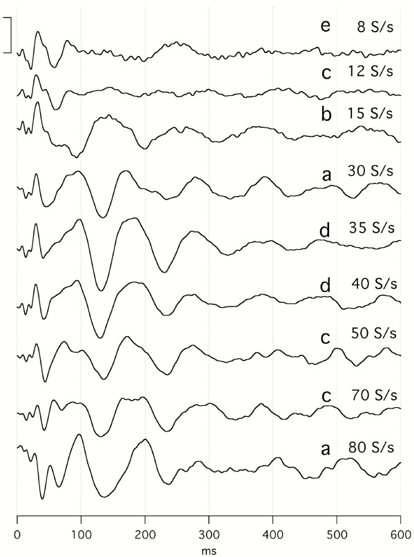
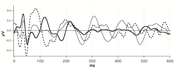
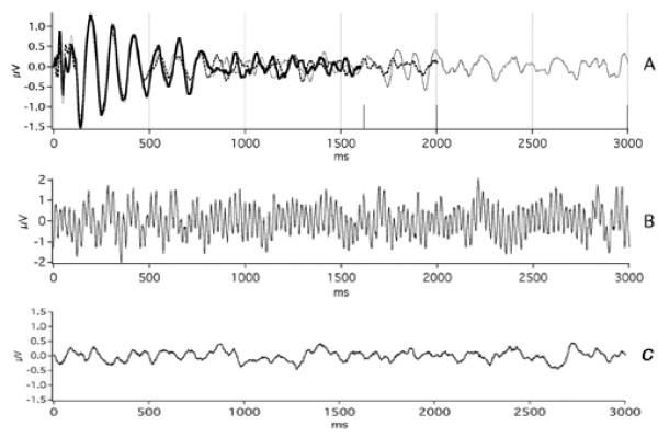
Background: A new method has been used to obtain human sensory evoked-responses whose time-domain waveforms have been undetectable by previous methods. These newly discovered evoked-responses have durations that exceed the time between the stimuli in a continuous stream, thus causing an overlap which, up to now, has prevented their detection. We have named them "A-waves", and added a prefix to show the sensory system from which the responses were obtained (visA-waves, audA-waves, somA-waves).

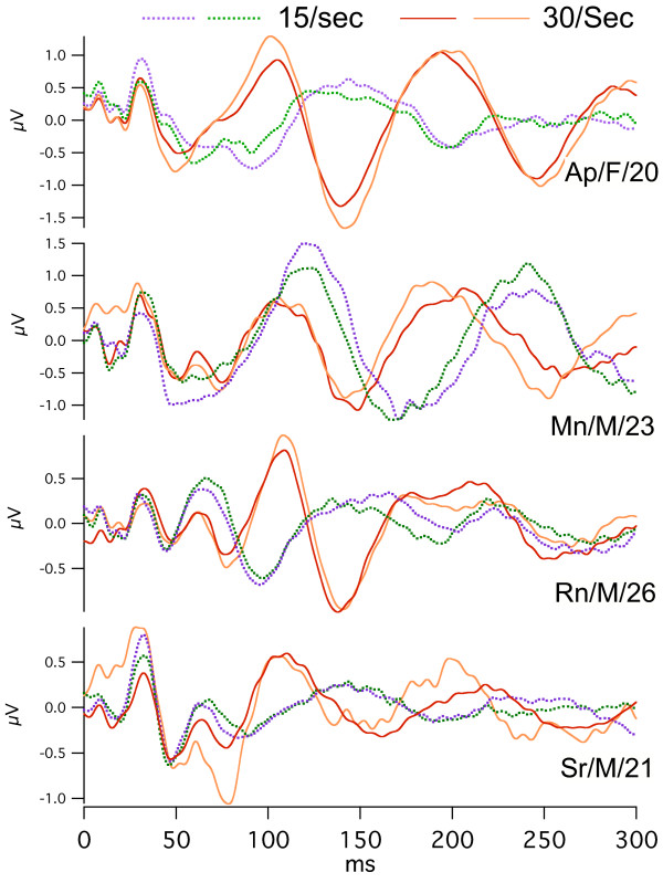
Results: When A-waves were studied as a function of stimulus repetition-rate, it was found that there were systematic differences in waveshape at repetition-rates above and below the psychophysical region in which the sensation of individual stimuli fuse into a continuity. The fusion phenomena is sometimes measured by a "Critical Fusion Frequency", but for this research we can only identify a frequency-region [which we call the STZ (Sensation-Transition Zone)]. Thus, the A-waves above the STZ differed from those below the STZ, as did the sensations. Study of the psychophysical differences in auditory and visual stimuli, as shown in this paper, suggest that different stimulus features are detected, and remembered, at stimulation rates above and below STZ.

Conclusion: The results motivate us to speculate that: 1) Stimulus repetition-rates above the STZ generate waveforms which underlie "fusion-memory" whereas rates below the STZ show neuronal processing in which "flash-memory" occurs. 2) These two memories differ in both duration and mechanism, though they may occur in the same cell groups. 3) The differences in neuronal processing may be related to "figure" and "ground" differentiation. We conclude that A-waves provide a novel measure of neural processes that can be detected on the human scalp, and speculate that they may extend clinical applications of evoked response recordings. If A-waves also occur in animals, it is likely that A-waves will provide new methods for comparison of activity of neuronal populations and single cells.

Figure 1

Diagram of QSD process. (Previously published [14].)

Figure 2

ABR recordings from two subjects. Taken from original paper [14]. Click stimuli delivered monaurally by Etymotic ER-2 insert-earphone at time '0' so that the stimuli arrive at the eardrum 1 ms later, due to tube-delay. A: ABR from male subject, clicks at 60 dbSL, at 55 S/s using a jittered sequence. The smallest SI in the sequence was 16 ms. The waveform found by QSD is the solid line. The dotted line is the 10 ms duration 'standard' average of the same data, triggered on each stimulus (no QSD). The similarity of waveforms shows that QSD returns the same waveform in a direct comparison (when there is no overlap). The passband was 120 to 2500 Hz. B: Recordings from female subject, clicks intensity 65 dbSL (relative to threshold measured at slowest rate). Passband filtered from 120 to 2000 Hz during deconvolution. At 9.6 S/s and 40 S/s waveforms obtained by standard averaging, one stimulus per sweep. Other traces obtained via QSD. Vertical dashed lines mark: (1) the timing of peak of the negative-going onset of the cochlear microphonic (CM) and (2) the peak of wave V. Note that the onset CM does not change latency with change in repetition-rate, but wave V does. C: The first part of the overlapped data from which the respective recordings in B were deconvolved (different time-scale). Note that absence of any 6 ms long flat portions in the convolved data, as compared with the pre-stimulus baseline in the deconvolved waveforms on the left.

Figure 3

G-wave auditory evoked-response recordings. Modified figure from [69]. Recorded from one electrode pair: C3 to right earlobe. Above: G0 peak of G-waves (solid line; passband 30–120 Hz) compared with the ABR (dashed line; passband 120–3000 Hz). Below: G-waves, on the same time scale as in A, but with a different vertical scale. Note: The peak of G0 corresponds to the middle of the ABR.

Figure 4

visA-waves recorded to a flash to the left visual hemifield, at various rates of stimulation. Sequence length = 1600 ms. Subj = Cg. Vertical scale = 4 V. Passband = 8–50 Hz. To see the convolved, averaged data from which this data was deconvolved follow this link: [see Additional file 6].

Figure 5

Same as Fig. 4, re-graphed with different vertical scales and with added latencies.

Figure 6

visA-waves recorded to a flash to the right visual hemifield, at various rates of stimulation. Sequence length = 1600 ms. Subj = Cg. Vertical scale = 4 V. To see the convolved, averaged data from which this data was deconvolved follow this link: [see Additional file 7].

Figure 7

Same as Fig. 6, re-graphed with different vertical scales and with added latencies.

Figure 8

audA-waves over a range of stimulus repetition-rates, in a single subject (Ap). Full data 1600 ms long; only first 300 ms shown. Monaural right stimulation at 65 dBSL. Abscissa, ms; ordinate bar = 1 V. Filter 8–50 Hz. On the right, the letters a-e refer to the dates on which the data were taken. The number of days between recordings are as follows: a-b, 8; b-c, 85; c-d, 7; d-e, 27. To see the convolved, averaged data from which this data was deconvolved follow this link: [see Additional file 8].

Figure 9

audA-waves from four subjects. Subject identifiers = code/gender/age. Recorded from the C3'-O2 channel, at two repetition-rates: 15 S/s (dotted lines) and 30 S/s (solid lines), with overlapping of replicate runs at each rate. The jitter maximum was 12% around the mean. Monaural, right ear, Etymotic tubephone stimulation. Abscissa, ms; ordinate V; Filter: 5–120 Hz. Averaged data before deconvolution 1600 ms long; only the first 500 ms are shown. Note that the vertical scales differ between subjects.

Figure 10

Day-to-day differences in audA-waves at two different repetition-rates in subject Ap. Monaural stimulation, right ear. The recordings were first taken over 15 days, and then 3 months later were taken over 42 days. The 15 S/s data shows 12 overlapped traces/days, and the 30 S/s data shows 9 traces/days. All traces are dotted, with the exception of the two traces having a maximum or minimum at 100 ms (to show how the same trace differs at other latencies). Note that despite the day-to-day variation, the polarities are opposite at about 100 ms, about 140 ms, about 200 ms, and about 250 ms.

Figure 11

Somatosensory A-waves (somA-waves) compared with visA-waves and audA-waves in the same subject. A: A single visA-wave run, stimulating the left hemifield. B: audA-waves at two different rates. Monoaural stimulation in right ear, Dau-chirps at 45 dBSL. C: somA-waves from right median nerve stimulation sufficiently strong to cause thenar muscle contraction. Replicate runs are shown at two different rates. Note: this male subject was 74 yrs old, and had some high-frequency hearing loss.

Figure 12

Comparison of a published "afterpotential" waveform and a visA-waveform, on two different time scales. A: "Classic" afterpotential, as shown on pg.379 of Regan's book [70], originally from Ciganek [71]. B: A visA-wave taken at 30 S/s. This is the same as shown in Fig. 4 but is plotted on the two different time scales of A.

Figure 13

Responses from trains of sinusoidally-varying light with a modulation depth of 10%, at rates near that of alpha waves. (Copied from Tweel, et al. [17].) Recordings in two subjects, at 11 Hz for Subject A, and 10 Hz for Subject B. The upper traces show the decay of response at the end of the train. The lower traces show the response build-up at the start of the train. Subject B shows much longer build-up and decay than does Subject A, and larger waves as well.

Figure 14

Diagram of the method used to compare A-waves. This is a diagram of the method used to compare: 1) the response to the second stimulus in paired-stimuli, and 2) the deconvolved response from QSD at the same SI. The goal is to determine the waveform at the start of a stimulus train, compared with the asymptotic response in the middle of the train. To make the comparison, the mean period in the QSD sequence is the same as the time between the two stimuli in the pair. A: The response to a pair of stimuli, where the response to the second stimulus of the pair is different from the response to the first stimulus. B: The response to a single stimulus. C: B subtracted from A gives just the response to just the second stimulus. D: C is moved to the left so as to ease the comparison with A. Note the time-scale has moved, but the time of stimulation for this response is now at the beginning of the sweep, as it is in B. E: The response to a single stimulus in a continuous stimulation at a repetition-rate with a period the same as in A. This waveform was deconvolved by QSD from overlapped data.

Figure 15

Demonstration that A-waves are not immediately generated by the first pair in the run. Abscissa, ms; ordinate V. Solid trace: The response to a single Dau-chirp presented at 15 S/s using a q- sequence. Dotted trace: The response to the second of a pair of Dau-chirps with the timing between the pair at 14 ms (the period of 70 S/s). The timing from start-of-pair to start-of-pair was 15 S/s, using the same q-sequence. See text for the method of extracting and shifting this waveform. Dashed trace: The response to the same Dau-chirps when they are presented in a jittered q-sequence, mean of 70 S/s. NOTE: The dotted trace is mid-way between the solid and dashed traces within the first 120 ms, i.e., the response to the second stimulus of the pair does not equal the response to continuous stimulation.

Figure 16

Control recordings when the flash was covered with cardboard. Vertical scale = 4 V. Top trace: Averaged EEG with no stimulus. Bottom trace: The deconvolved average of the top trace (no response).

Figure 17

audA-wave data from subject Mn. Monaural right ear stimulation. Abscissa, ms; ordinate V; Filter: 5–130 Hz. Full data length shown. Top trace: audA-waves from stimulation at 40 S/s taken on three separate Sequence Lengths: 1.6 s, 2 s, 3 s. Note that up to about 500 ms the waveforms overlay with only small differences. From 500 to perhaps 1400 ms there is some agreement, but clearly there are more differences. Middle trace: Overlapped (convolved) data from which the 3 s waveform in the Top trace was deconvolved. There are 20 stimuli every 500 ms. Bottom trace: Control EEG obtained without stimulation, then averaged, and deconvolved. Note absence of any "response".

Figure 18

A-waves to either visual or auditory stimulation, using the same q-sequence. Abscissa: ms; ordinate V. Flash traces are inverted to correspond to VEP convention. A: visA-waves to flashes at 40 S/s. Male subject, Bt, 17 yrs. NOTE the ordinate – the visual responses are much larger than auditory responses. B: audA-waves to Dau-chirps at 40 S/s, same timing sequence and same subject as in A. NOTE that there are differences at short latencies (no G-waves in A), and in the duration of the A-wave oscillations. NOTE that the "jaggedness" of this trace may be due to the increased gain, as compared with A. C: audA-waves to Dau-chirps at 40 S/s, same sequence as in B but the subject is different (Male subject, Ma, 26 yrs).

Figure 19

The effect of filtering on the overall shape of audA-waves and visA-waves. A: Subject = Mn. Monaural right ear stimulation at 40 S/s. Abscissa, ms; ordinate V. The sequence-length was 3 sec, of which only the first 1500 ms are shown. Run time = 100 min (1 hr, 40 min). Dotted lines = Data passband filtered 1–120 Hz. Solid lines = The same data filtered 5–120 Hz. (Note that this is the only recording shown in this paper that shows data with the highpass filter down to 1 Hz.) The effect of the filter (solid line) is to create a monotonic descent of the peak heights, which appears as a damped sinusoid, but that the brain's response (dotted line) actually has an increased positive peak just before 200 ms, and an increased negative valley at about 375 ms. The waves after about 475 ms have a magnitude within the noise level of the rest of the sweep (1000–3000 ms – not shown). Note also the filtered waveform (solid line) is more regular than the 1–120 Hz data (dotted line). B: Subject = Cg. Flash stimuli, left visual hemifield, 30 S/s. Same data as Fig. 12. Dotted Lines = Data passband filtered 5–120 Hz. Solid Line = The same data as the Dotted Line, but passband filtered 8–50 Hz. The differences due to the narrower passband are small – some are indicated by arrows.

Figure 20

Demonstration of the effects of rate of visual stimulation on detection of image changes. A: Steady presentation of a field of light gray disks on a slightly darker background. B: Same as A except the disks are flashed at a rate of 2.4 S/s and one of the disks is moving an amount equal to its radius. [click "MovieB" below to see this]. C: Same video frames as in B except presented at a rate of 12 S/s (same as frame rate of movie) [click "MovieC" below to see this] MovieB [see Additional file 12] MovieC [see Additional file 5]

Figure 21

Limulus eye study, showing the effect of a step-increase in illumination to ommatidium "A". Modified from [72].

Figure 22

Sounds of different auditory stimuli, at different repetition-rates and at different percentage-jitters. The following files produce clicks that are at uniform rate, where the number is S/s. 2persec_click [see Additional file 17] 4persec_click [see Additional file 19] 6persec_click [see Additional file 21] 8persec_click [see Additional file 23] 10persec_click [see Additional file 25] 12persec_click [see Additional file 27] 14persec_click [see Additional file 29] 16persec_click [see Additional file 31] 18persec_click [see Additional file 33] 20persec_click [see Additional file 35] 22persec_click [see Additional file 37] 24persec_click [see Additional file 39] 26persec_click [see Additional file 41] 28persec_click [see Additional file 43] 30persec_click [see Additional file 45] 40persec_click [see Additional file 47] 50persec_click [see Additional file 49] 70persec_click [see Additional file 51] 90persec_click [see Additional file 53] 100persec_click [see Additional file 55] The following audio files produce Dau-chirps that are at uniform rate, where the number is S/s. Same repetition-rates as for click's, above. 2persec_dau [see Additional file 18] 4persec_dau [see Additional file 20] 6persec_dau [see Additional file 22] 8persec_dau [see Additional file 24] 10persec_dau [see Additional file 26] 12persec_dau [see Additional file 28] 14persec_dau [see Additional file 30] 16persec_dau [see Additional file 32] 18persec_dau [see Additional file 34] 20persec_dau [see Additional file 36] 22persec_dau [see Additional file 38] 24persec_dau [see Additional file 40] 26persec_dau [see Additional file 42] 28persec_dau [see Additional file 44] 30persec_dau [see Additional file 46] 40persec_dau [see Additional file 48] 50persec_dau [see Additional file 50] 70persec_dau [see Additional file 52] 90persec_dau [see Additional file 54] 100persec_dau [see Additional file 56] The following audio files show the effect of increasing the amount of jitter, using Dau-chirps at a mean rate of 40 S/s. The number indicates the percentage jitter. The uniform 40 S/s is also provided for convenience, as the "No jitter – uniform" file. The "MLS" Button is a Maximum-Length Sequence (= "m-sequence") of 511 stimuli, where the minimum interval is 25 ms (= 40 S/s). It is notable that as the jitter is increased, not only is the "tone" diminished, but the quality of the stimulus-sensation changes. We conjecture that a minimum number of consecutive SIs are needed before fusion-memory "locks in", and that larger jitter prevents this. "No jitter – uniform" [see Additional file 48] "12percent jitter" [see Additional file 58] "24percent jitter" [see Additional file 59] "36percent jitter" [see Additional file 60] "MLS" [see Additional file 57]

Figure 23

The quantal nature of frequency in auditory fusion. This is Fig. 7-49, on p. 260, of v. Bekesy's book [12].

Figure 24

Simulation of overlap of visA-waves at different repetition-rates. The black dotted lines are the same data as shown in Fig. 4. Each waveform is duplicated and moved to the right by a distance equal to the mean repetition-rate for that waveform. This is repeated 4 times, so that the overlap of 5 successive responses are shown. Note: that there are multiple places where the peak from one stimulus overlaps a different peak from a different stimulus. These could be locations at which a given neuron could not fire at the same phase of every cycle. Note further that this is a simulation because there is not SI jitter, and that only 5 of the responses are shown, whereas in the experiments the stimuli were continuously presented.

Figure 25

A nonlinear response is detected by repeated linear approximations by small excursions of the variable. (This figure taken from QSD methods paper [14].)

Figure 26

Frequency-domain plot of a visA-wave. The time-domain waveform is shown in Fig. 4, at 30 S/s. The 6 frequency-domain comb-filter amplitude plots at the bottom are those for uniform stimulus repetition-rates at the repetition-rates indicated.

Figure 27

Animated simulations: SS compared with QSD. Herein you can access 6 simulations, 3 each for SS and for QSD. There are three ranges of mean repetition-rate: A = 0.3 – 2.4 S/s. B = 3 – 11 S/s. C = 11 – 25 S/s. Each of these rates can be seen for either SS or QSD from the following Demonstration files:"Fig. 27_SS_A" [see Additional file 13]"Fig. 27_SS_B" [see Additional file 14]"Fig. 27_SS_C" [see Additional file 15]"Fig. 27 QSD_A" [see Additional file 9]"Fig. 27 QSD_B" [see Additional file 10]"Fig. 27 QSD_C" [see Additional file 11] SS Animations These animations contain simulations of SS responses based upon an actual brain response waveform, also seen in Fig. 4, 30 S/s. That response is shown as a red trace in the lower left-hand side of all the steady-state animations. Above that is shown a 500 ms SS response in black, this is the same epoch length as used by Herrmann [16] and is equivalent to his averaged SS responses. The long blue trace shows the convolution of the brain response shown in the lower left, with a periodic sequence at the rate shown by the number in the top left. The first five seconds of our simulated convolved response are shown in the upper blue trace. In the bottom right hand corner there is a box that contains information plotted in the frequency domain. This box contains the frequencies from 0 Hz to 26 Hz with a mark below the horizontal axis showing 10 Hz. The red trace in the box is the magnitude of the Fourier coefficients of the time-domain brain response shown in the bottom left red trace. The blue dots are the Fourier coefficients of the blue trace above. The black vertical lines are the Fourier magnitudes of the periodic sequence (comb filter) with which the brain response is convolved. NOTE: All of the traces in these animations may have been scaled, and/or cropped for demonstrative purposes. QSD Animations These animations contain simulations of QSD responses based upon an actual brain response wave form recovered with the QSD method, also seen in Fig.4, 30 S/s. This response is shown in red at the bottom left. The long blue trace in the middle of the animation is the convolution of the brain response shown, with a QSD sequence at the mean repetition rate shown by the number in the top left. This trace is equivalent to our data-averages when stimulating with a QSD sequence. It is 5 sec long (longer than we have ever used) in order to show, in the simulation of the lowest stimulus repetition-rates the gradual overlap of the individual responses. In the bottom left, above the red trace is shown, in black, the corresponding waveform deconvolved from the upper blue trace (after random noise had been added). If we had not added noise here there would be no changes in the deconvolved trace during the animation. (Each of the three animations was based upon a different QSD sequence. QSD sequences for these simulations were produced by taking a QSD sequence used in this paper (see Table 1 [see Additional file 16]) and using it for multiple stimulus repetition-rates. To accomplish this author MO changed the sampling rate used during the simulation. (The frequencies are thinning as the repetition-rate goes faster in the animation because we did not want to find so many good q-sequences. So in the simulation, the use of one q-sequence over multiple frequencies led to automatic change in the length of the convolved data with every change in stimulus repetition-rate. This had the consequence that the number of frequencies analyzed changed, and this appears as changing q-sequence frequencies during the animation. In actual practice, since the SL is often the same length even though the repetition-rate is changed, the frequencies in the deconvolution waveformare the same.) In the bottom right hand corner there is a box that contains information plotted in the frequency-domain. This box contains the frequencies from 0 Hz to 26 Hz with a mark below the horizontal axis showing 10 Hz. The red trace here is the magnitude of the Fourier coefficients of the brain's response shown in the red trace at the bottom left. The blue dots are the Fourier coefficients of the convolution shown as the blue trace above. The black vertical lines are the Fourier magnitudes of the q-sequence (i.e., Q-magnitudes) with which the brain's response is convolved (see QSD paper for further details) [14]. The tick marks on the vertical axis show the Q-magnitudes 1 and 5 of the q-sequence (cropped above 5). NOTE: All of the other traces in these animations may have been scaled, and/or cropped for demonstrative purposes.

References

1. Kompass R. Universal temporal structures in human information processing: a neural principle and psychophysical evidence. In: Kaernback C, Schroger E, Muller H, editor. Psychophysics Beyond Sensation: Laws and Invariants of Human Cognition. Mahwah, NJ: Lawrence Erlbaum Associates; 2004. pp. 451–480.
1. Lalanne L. Sur la duree de la sensation tactile [On the duration of tactile sensations] Note Comptes Rendus de l'Acadenue des Sciences Paris. 1876;39:1314–1316.
1. Brecher GA. The emergence and biological significance of the subjective time unit perceptual moment. (in German: Die Entstehung und biologische Bedeutung der subjektiven Zeiteinheit – des Moments. Zeitschrift fur vergleichende Physiologie. 1932;18:204–243.
1. Maskin MB, Riklan M, Chabot D. Effects of "short-term" versus "long-term" L-Dopa therapy in parkinsonism on critical flicker frequency. Percept Mot Skills. 1974;38:455–458. - PubMed
1. Riklan M, Levita E, Misiak H. Critical flicker frequency and integrative functions in parkinsonism. J Psychol. 1970;75:45–51. - PubMed
Publication types