Local osmosis and isotonic transport

Abstract

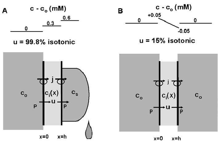
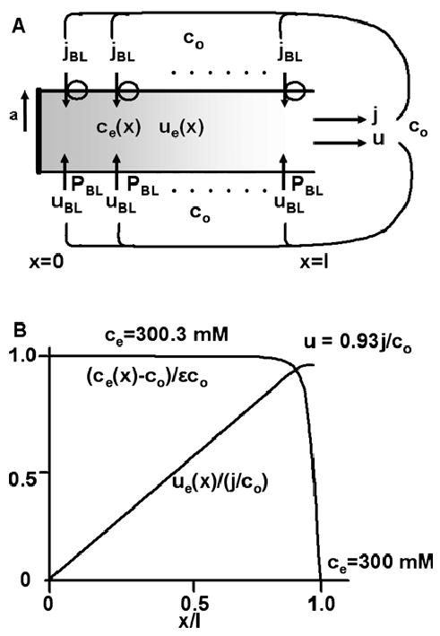
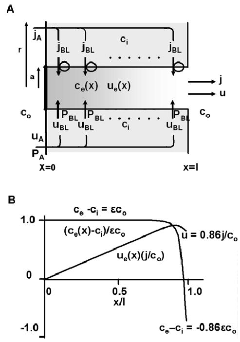
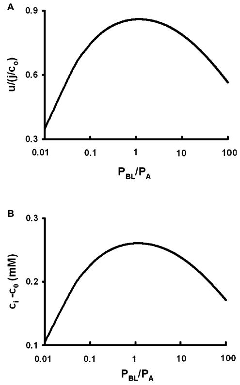
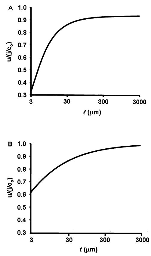
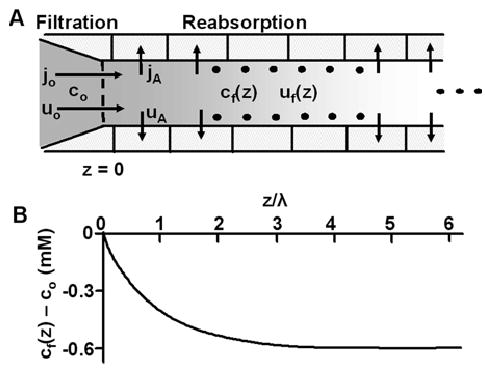
Osmotically driven water flow, u (cm/s), between two solutions of identical osmolarity, c(o) (300 mM: in mammals), has a theoretical isotonic maximum given by u = j/c(o), where j (moles/cm(2)/s) is the rate of salt transport. In many experimental studies, transport was found to be indistinguishable from isotonic. The purpose of this work is to investigate the conditions for u to approach isotonic. A necessary condition is that the membrane salt/water permeability ratio, epsilon, must be small: typical physiological values are epsilon = 10(-3) to 10(-5), so epsilon is generally small but this is not sufficient to guarantee near-isotonic transport. If we consider the simplest model of two series membranes, which secrete a tear or drop of sweat (i.e., there are no externally-imposed boundary conditions on the secretion), diffusion is negligible and the predicted osmolarities are: basal = c(o), intracellular approximately (1 + epsilon)c(o), secretion approximately (1 + 2epsilon)c(o), and u approximately (1 - 2epsilon)j/c(o). Note that this model is also appropriate when the transported solution is experimentally collected. Thus, in the absence of external boundary conditions, transport is experimentally indistinguishable from isotonic. However, if external boundary conditions set salt concentrations to c(o) on both sides of the epithelium, then fluid transport depends on distributed osmotic gradients in lateral spaces. If lateral spaces are too short and wide, diffusion dominates convection, reduces osmotic gradients and fluid flow is significantly less than isotonic. Moreover, because apical and basolateral membrane water fluxes are linked by the intracellular osmolarity, water flow is maximum when the total water permeability of basolateral membranes equals that of apical membranes. In the context of the renal proximal tubule, data suggest it is transporting at near optimal conditions. Nevertheless, typical physiological values suggest the newly filtered fluid is reabsorbed at a rate u approximately 0.86 j/c(o), so a hypertonic solution is being reabsorbed. The osmolarity of the filtrate c(F) (M) will therefore diminish with distance from the site of filtration (the glomerulus) until the solution being transported is isotonic with the filtrate, u = j/c(F).With this steady-state condition, the distributed model becomes approximately equivalent to two membranes in series. The osmolarities are now: c(F) approximately (1 - 2epsilon)j/c(o), intracellular approximately (1 - epsilon)c(o), lateral spaces approximately c(o), and u approximately (1 + 2epsilon)j/c(o). The change in c(F) is predicted to occur with a length constant of about 0.3 cm. Thus, membrane transport tends to adjust transmembrane osmotic gradients toward epsilonc(o), which induces water flow that is isotonic to within order epsilon. These findings provide a plausible hypothesis on how the proximal tubule or other epithelia appear to transport an isotonic solution.

Fig. 1

The main components of transmembrane osmosis. Bulk solution is assumed to have osmolarity c_o, with possible local gradients of order Δc. Salt is actively transported across the membrane at a rate j nd water follows by osmosis at a rate u through an independent pathway, primarily via aquaporins. The presence of aquaporins confers a specific membrane osmotic permeability P, so the rate of fluid transport is determined by u = PΔc.

Fig. 2

A simple two-membrane model of epithelial transport. (A) Secretion of fluid without boundary conditions on the secretion. The basolateral membranes are washed with a well-stirred solution of osmolarity c_o; the intracellular osmolarity C_i(X) is allowed to vary across the epithelium, but the calculations suggest it is essentially constant because difiusion is very effective over short distances; the secreted solution has osmolarity c_s, which is determined by the membrane water permeability and the rate of salt transport, j. Since the flux of salt in the secretion is carried entirely by convection, it is given by j = uc_s. Hence the boundary condition on the osmolarity of the secretion is c_s = j/u for model A. (B) The same simple model of an epithelium, but now each side is washed with a well-stirred solution whose osmolarity is c_o. Thus the difference in the two models is the boundary condition on the secretion, which is c_s = c_o for model B.

Fig. 3

A tube of transporting membrane immersed in a solution of osmolarity c_o. This model has been used to represent the lateral intercellular spaces of a transporting epithelium (Diamond & Bossert, 1967). (A) The geometric and transport properties of the tube. The transmembrane salt flux, j_BL, is assumed to be uniform along the lateral membrane. This leads to a longitudinal flux j_e(x) (moles/cm²/s) that increases linearly with distance from the apical junction (x = 0), which is assumed to be impermeable to solute or fluid. Local osmotic gradients c_e(x) (moles/cm³) generate transmembrane water flow u_BL(x) (cm/s) and cumulative longitudinal water flow u_e(x) (cm/s). The emerging solution has osmolarity j/u, where u = u_e(l) and j = 2πal j_BL. At the end of the tube, c_e(l)= c_o The transport equations are derived in the text, where approximate solutions are presented. (B) Graphical representations of the solutions to the transport equations. The normalized concentration gradient and water flow are graphed. The calculated values of the concentration of solute along the majority of the tube and just at the end of the tube are indicated on the graph.

Fig. 4

A cellular model of epithelial transport. (A) The geometric and transport properties of the cellular transport model. The properties of the lateral intercellular spaces are the same as described in Fig.3. The cellular dimension r (cm) is chosen so that the area of apical membrane relative to basolateral membrane is appropriate for the tissue of interest (see text). The new feature of this model is the osmolarity of the intracellular compartment, c_i (moles/cm³), which is determined such that apical and basolateral membrane water fluxes are the same. In addition, apical and basolateral membrane solute fluxes are constrained to be the same, implying πr²j_A = 2πal j_BL. The transport equations are derived in the text, where approximate solutions are presented. (B) Graphical representations of the solutions to the transport equations. The normalized concentration gradient and water flow are graphed. The calculated values of the concentration of solute along the majority of the tube and just at the end of the tube are indicated on the graph.

Fig. 5

The effect of increasing basolateral membrane water permeability (P_BL), with all else constant. The calculations are based on the cellular model shown in Fig. 4. (A) The rate of fluid transport as a function of P_BL. Fluid transport is maximum when total apical and basolateral water permeabilities are equal: πr²P_A = 2πal P_BL. (B) The osmotic gradient across apical membranes as a function of P_BL. As P_BL decreases, basolateral water flow becomes rate limiting and the concentration of solute in the cell decreases to reduce apical flow and maintain balance. As P_BL increases, the concentration of solute in the lateral spaces and the cell approach c_o, causing the apical transmembrane osmotic gradient to decrease and apical flow becomes rate limiting.

Fig. 6

The effect of increasing the length of lateral spaces as in layered epithelia or the lens. To maintain equality of salt transport, we set πr²j_A = 2πal j_BL by reducing j_BL in proportion to 1/l, with j_A constant. (A) Fluid transport as a function of l when apical and basolateral membrane water permeabilities are maintained constant. Because the boundary condition effect at the mouth of the tube reduces net transport (see text describing Fig. 4A), the longer the cleft the less important this effect and transport increases. However, because increasing cleft length also has the effect of increasing total basolateral membrane water permeability relative to apical, eventually apical water transport becomes rate limiting and water transport never exceeds 92% isotonic. (B) Fluid transport as a function of l when apical and basolateral membrane water permeabilities are maintained equal by reducing P_BL as 1/l. In this situation, the mouth of the tube effect becomes negligible at long l, but apical flow does not become rate limiting, hence water transport approaches its isotonic limit.

Fig. 7

Fluid and salt reabsorption in the renal proximal tubule. (A) The geometric and transport properties of the proximal tubule. The new filtrate c_f= c_o (moles/cm³) is generated by the glomerulus at z = 0. As the filtrate flows along the lumen of the tubule, salt is transported out of the tubule across apical membranes at a rate j_A (moles/cm²/s) and water follows at a rate u_A (cm/s). The osmolarity of the transported solution, j_A/u_A (moles/cm³), is initially c_o/0.86 (Eq. 22 and related text), implying c_f is decreasing with increasing distance from the glomerulus. The transport equations are derived in the text, where approximate solutions are presented. (B) A graphical representation of the solution for c_f as a function of distance from the glomerulus. Based on parameter values in Table 2, ε = 10⁻³ and the total water permeabilities of apical and basolateral membranes are the same, hence α = 1. Initially c_f = c_o = 300 mM, but it exponentially declines to its steady-state value of (1−(1+α)ε)c_o = 399.4 mM with a length constant λ = 0.3 cm. At steady state, the osmolarities of the transported solution and the filtrate are the same: c_f = j_A/u_A.

References

1. Barfus DW, Schafer JA. Rate formation and composition of absorbate from proximal nephron segments. Am J Physiol. 1984;247:F117–F129. - PubMed
1. Curran PF. Na, Cl, and water transport by rat ileum in vitro. J Gen Physiol. 1960;43:1137–1148. - PMC - PubMed
1. Curran PF, Mclntosh JR. A model system for biological water transport. Nature. 1962;193:347–348. - PubMed
1. Diamond JM. The mechanism of isotonic water transport. J Gen Physiol. 1964;48:15–42. - PMC - PubMed
1. Diamond JM, Bossert WH. A mechanism for coupling of water and solute transport in epithelia. J Gen Physiol. 1967;50:2061–2083. - PMC - PubMed
Publication types
Substances
LinkOut - more resources