Linear-Nonlinear-Poisson models of primate choice dynamics

Abstract

The equilibrium phenomenon of matching behavior traditionally has been studied in stationary environments. Here we attempt to uncover the local mechanism of choice that gives rise to matching by studying behavior in a highly dynamic foraging environment. In our experiments, 2 rhesus monkeys (Macacca mulatta) foraged for juice rewards by making eye movements to one of two colored icons presented on a computer monitor, each rewarded on dynamic variable-interval schedules. Using a generalization of Wiener kernel analysis, we recover a compact mechanistic description of the impact of past reward on future choice in the form of a Linear-Nonlinear-Poisson model. We validate this model through rigorous predictive and generative testing. Compared to our earlier work with this same data set, this model proves to be a better description of choice behavior and is more tightly correlated with putative neural value signals. Refinements over previous models include hyperbolic (as opposed to exponential) temporal discounting of past rewards, and differential (as opposed to fractional) comparisons of option value. Through numerical simulation we find that within this class of strategies, the model parameters employed by animals are very close to those that maximize reward harvesting efficiency.

Figure 1. (A) Schematic depiction of the foraging task.

Subjects alternately view a presentation screen where they must hold their gaze on a central fixation marker (cross), and a choice screen where they are free to direct their gaze to either of the two colored targets, one red and one green. Rewards are delivered on dynamic VI schedules. (B) Schematic diagram of the process governing the state of a single target. Empty targets have a constant probability per unit time of being baited. Once baited, targets only become unbaited when the animal chooses said target and collects the reward. (C) Block-wise matching behavior for each of the 2 monkeys in our study. Each data point represents a block of trials on which the baiting probabilities for each target were held constant. Reward and choice fraction are shown here, and in all subsequent figures, relative to the red target (for the green target, the equivalent metrics are one minus the value for the red target). Thus the abscissa in 1C denotes the fraction of the total rewards in a particular block that were earned on the red target. (D) The same data from 1C is replotted as the log of the ratio of choices made to (or the rewards earned on) the two targets in each block. Blocks for which no rewards were earned on one or the other color are omitted to avoid data at +/− infinity. The data are fit by linear regression (solid line); the insets show the equation for the generalized matching law and the parameters of the fitted regression line.

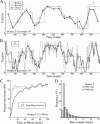
Figure 2. (A) Time-course of reward and choice fractions for a single experiment.

The thin line shows the fraction of the total baiting probability assigned by the experimenter to the red target. The dashed line shows the resulting experienced reward fraction for the red target, calculated for the first, middle, and last third of each block. The thick line shows the animal's choice fraction for the red target over the same period. (B) High temporal resolution view of reward and choice fraction time-courses. The data are the same as in A, but with reward and choice fractions computed locally using a Gaussian filter (inset), rather than chunked by thirds of a block. (C) Behavioral response to block transitions. The dashed and solid curves plot the average time-course of adaptation of reward and choice fractions after a block transition, in normalized units where the fractional baiting probability on the previous block is 0% and the fractional baiting probability on the new block is 100%. Reward and choice fractions are computed using a box filter (inset) before averaging across blocks. (D) Distribution of run lengths for Monkey F across all experiments. Each bin shows the relative frequency of choosing a target exactly n consecutive times before returning to the other option.

Figure 3. Diagram of a generic LNP model for choice.

Past rewards enter at the left, coded as a binary stream. A linear filter weights the rewards based on their distance in the past. The resulting scalar is mapped to probability of choice by a low-dimensional nonlinear function. That probability of choice is then used to drive an inhomogeneous Poisson process, which in turn renders the ultimate binary choice.

Figure 4. (A) Filters estimated for the L-stage of our LNP model.

The points indicate the raw filter weights recovered by Wiener kernel analysis for each monkey. These weights show the relative influence of rewards earned on each of the last 50 trials on the animal's subsequent choice. The filters are normalized so that the recovered weights sum to 1.0. The solid line shows the best double exponential fit to these raw filter weights; the inset shows the parameters that describe this double exponential. (B) Nonlinear decision criterion estimated for the N-stage of our LNP model. For each monkey, we show the relation between the scalar value metric, differential value, as computed by the L-stage filters shown in A, and the animals' ultimate probability of choice. The data points are equally populated bins showing the fraction of choices made to the red target for trials when the filtered reward stream held a particular value. Only free choices are included in computing these probabilities. The solid line shows the best-fitting cumulative Gaussian. Parameters describing this cumulative Gaussian are shown in the inset.

Figure 5. Diagram of our final parameterized LNP model.

Past rewards enter at the left, separately coded as a binary stream for each color. Rewards are coded as zeros if the animal did not choose the target on that trial, or if it chose the target but was not rewarded. Two identical double exponential filters weight these rewards based on their distance in the past. The difference of the output of these two filters is an intermediate scalar value metric we term differential value. Differential value is mapped to probability of choice by a sigmoidal decision function, parameterized as a cumulative Gaussian. That probability of choice is then used to drive an inhomogeneous Poisson process, which renders the ultimate binary choice.

Figure 6. Predictive performance of the model.

(A) The monkey's local choice fraction for this experiment is replotted from Figure 2B now as a dashed curve. The solid line shows the choice fraction predicted by the LNP model diagramed in Figure 5, using the parameters given for Monkey F in Figure 4. Predicted choice fractions are smoothed with the same filter used for the actual choice fractions, shown in the inset of Figure 2B. For reference, the experimenter-manipulated fractional baiting probabilities also are replotted from Figure 2B as the same thin solid line. (B) Overall predictive performance of the model. Using the model recovered for each monkey, we computed a predicted probability of choice on each free-choice trial in our entire data set. Based on these predictions, trials were then sorted into 30 equally populated bins. In each bin, we compute the probability of choice actually observed as the fraction of red target choices in each bin. The 95% confidence intervals on these estimates are smaller than the plotted points.

Figure 7. Generative performance of the model.

(A) This panel follows the conventions established in Figure 2B, but now shows local reward and choice fractions for synthetic behavior generated when the model diagrammed in Figure 5 performed the foraging task in simulation. The additional double-thickness line shows the average choice fraction over many repetitions of this block sequence using different random number seeds, thereby averaging out the noise in individual runs. (B) Adaptation dynamics. The curves in this panel are calculated as per Figure 2C. The dashed lines show the time-course of choice fraction adaptation for each monkey after a block boundary transition. The thick black lines show the same time-course computed from synthetic choice data generated by the model we recovered for each monkey; simulations were run on the same block sequences experienced by each monkey during our experiments. (C) Run length histograms for each animal, following the conventions established in Figure 2D. The thick black lines show the distribution of run lengths produced in the same monkey-specific simulations used to generate the data in Figure 2B. The inset shows these distributions in finer detail for very long run lengths.

Figure 8. Comparison of candidate N-stage nonlinearities.

Each panel shows a probability of choice surface as a function of the linear filter outputs for both targets. Thus the pixel in the upper left corner of each panel shows the probability of choosing the red target when the filtered reward history on the red target produces a value of 0.5 rewards and the filtered reward history on the green target produces a value of 0.0 rewards. The leftmost panel shows the probability of choice surface produced by the model diagrammed in Figure 5, where a sigmoidal nonlinearity operated on the difference of filter outputs (i.e., differential value). The second panel shows the probability of choice surface produced by a model that computes probability of choice by expressing the output of one filter as a fraction of the summed outputs of both (i.e., fractional value). The right two panels show the observed probability of choice surface that was actually observed for each of the 2 monkeys in our study. In these two panels, the filter output values were computed using the filter recovered for that particular animal (Figure 4A). Bins containing fewer than 10 free-choice trials are shown in white.

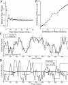
Figure 9. A choice-based model—an LNP model recovered for Monkey F that relates past choices, rather than past rewards, to future choice.

(A) L-stage filter, analogous to Figure 4A. (B) N-stage decision criterion, analogous to Figure 4B. (C) Predictive performance, analogous to Figure 6A. (D) Generative failure, analogous to Figure 7A.

Figure 10. Effect of unrewarded trials on model performance.

Rather than coding reward histories with ones for rewarded trials and zeros for all unrewarded trials, we code reward histories for each color with ones when that color was chosen and rewarded, δs when it was chosen and unrewarded, and zeros when it was not chosen. Positive δs indicate that unrewarded choices are reinforcing (having the same sign as rewards), whereas negative δs are frustrating (having the opposite sign). For each value of δ, we reestimated the LNP model for each monkey. (A) Effect of δ on the prediction of free choices for each monkey. (B) Effect of δ on the overlap between observed and generated run-length histograms for each animal.

Figure 11. (A) Effect of model parameters on reward harvesting.

From left to right, the three panels show the effect of varying τ₁, τ₂, and σ on reward harvesting efficiency. Harvesting efficiency is defined to be the average rewards earned per trial, normalized by the total baiting probability on both targets. Each point shows the harvesting efficiency of the best-performing model using the specified parameter value. Thus the leftmost point in the leftmost panel is the performance of the best model using a τ₁ of 1/16 of a trial, whereas τ₂ and σ are free to assume any value. (Note: Very small values of τ₁, e.g., 1/16, approximate the case where only the first trial is given nonzero weight.) Each point represents the average harvesting efficiency of this best-performing model over 10 repetitions of our entire data set, using different random-number seeds for each repetition. Arrows indicate the parameter values recovered in Figure 4 for each monkey. (B) Cross sections through the volume showing harvesting efficiency as a function of all three parameters. From left to right, the three panels show a plane with constant τ₁, τ₂, and σ, respectively. The value of the fixed parameter is shown in the inset. Harvesting efficiency for all combinations of the other two parameters is shown color coded from blue (poor harvesting efficiency) to red (high harvesting efficiency).

Figure 12. Regressions of neural data onto two different value metrics.

For each of 62 neurons recorded by Sugrue, Corrado, and Newsome (2004) in the same 2 animals whose behavioral data are presented here, we plot the unsigned Pearson's correlation coefficient relating each of two putative value metrics to changes in neural firing rate preceding choices both into and out of the cell's response field. Fractional value, the value metric in the original study, is shown on the abscissa and differential value, the hidden variable in the LNP model presented here, is shown on the ordinate. Regressions that were statistically significant (p < 0.05) for both decision variables are plotted as filled circles, those that were significant for one but not both are plotted as shaded circles, and those that were not significant for either are shown as open circles.

Figure A1. (A) Kernel estimation stability.

The top half of the panel diagrams the procedure used. Starting from raw behavioral data obtained from a particular animal, a linear filter was reconstructed using Wiener kernel analysis. This raw kernel was then fit with a double exponential, shown by the solid line (bottom panel). Artificial data were generated in simulation using this fit kernel, and then a new kernel was reconstructed from these artificial data. This repeated estimate of the kernel is shown in the open data points (bottom panel). (B) Arbitrary kernel estimation. An arbitrary linear filter (the solid line in the bottom panel) was used to generate synthetic data in simulation as diagrammed in the top half of the panel. These data were generated using the same block sequences, and were of the same size, as those presented to the monkeys in actual behavioral experiments. The open data points (bottom panel) show the recovered estimate of the underlying filter based on these artificial data. Recovered kernels in both A and B fit the input kernels quite well.

References

1. Barraclough D.J, Conroy M.L, Lee D. Prefrontal cortex and decision making in a mixed-strategy game. Nature Neuroscience. 2004;7:404–410. - PubMed
1. Baum W.M. On two types of deviation from the matching law: Bias and undermatching. Journal of the Experimental Analysis of Behavior. 1974;22:231–242. - PMC - PubMed
1. Baum W.M. Matching, undermatching, and overmatching in studies of choice. Journal of the Experimental Analysis of Behavior. 1979;32:269–281. - PMC - PubMed
1. Baum W.M. Optimization and the matching law as accounts of instrumental behavior. Journal of the Experimental Analysis of Behavior. 1981;36:387–403. - PMC - PubMed
1. Baum W.M. Choice, changeover, and travel. Journal of the Experimental Analysis of Behavior. 1982;38:35–49. - PMC - PubMed
LinkOut - more resources