Neural variability in premotor cortex provides a signature of motor preparation

Abstract

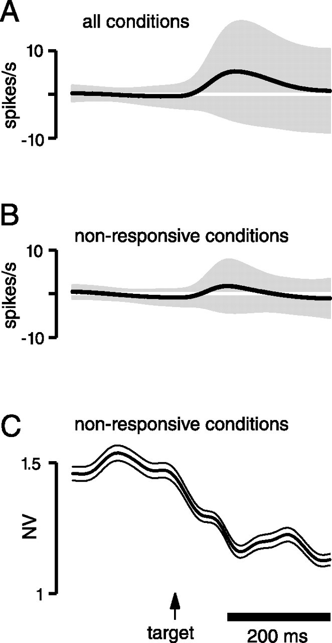
We present experiments and analyses designed to test the idea that firing rates in premotor cortex become optimized during motor preparation, approaching their ideal values over time. We measured the across-trial variability of neural responses in dorsal premotor cortex of three monkeys performing a delayed-reach task. Such variability was initially high, but declined after target onset, and was maintained at a rough plateau during the delay. An additional decline was observed after the go cue. Between target onset and movement onset, variability declined by an average of 34%. This decline in variability was observed even when mean firing rate changed little. We hypothesize that this effect is related to the progress of motor preparation. In this interpretation, firing rates are initially variable across trials but are brought, over time, to their "appropriate" values, becoming consistent in the process. Consistent with this hypothesis, reaction times were longer if the go cue was presented shortly after target onset, when variability was still high, and were shorter if the go cue was presented well after target onset, when variability had fallen to its plateau. A similar effect was observed for the natural variability in reaction time: longer (shorter) reaction times tended to occur on trials in which firing rates were more (less) variable. These results reveal a remarkable degree of temporal structure in the variability of cortical neurons. The relationship with reaction time argues that the changes in variability approximately track the progress of motor preparation.

Figure 1.

Illustration of the optimal-subspace hypothesis. The configuration of firing rates is represented in a state space, with the firing rate of each neuron contributing an axis, only three of which are drawn. For each possible movement, we hypothesize that there exists a subspace of states that are optimal in the sense that they will produce the desired result when the movement is triggered. Different movements will have different optimal subspaces (shaded areas). The goal of motor preparation would be to optimize the configuration of firing rates so that it lies within the optimal subspace for the desired movement. For different trials (arrows), this process may take place at different rates, along different paths, and from different starting points.

Figure 2.

Simulations illustrating how an increasing consistency in across-trial firing rate could be detected using the NV metric. Simulations were based on the mean firing rate of one recorded neuron (solid black trace at top). Baseline activity was artificially extended (to the left) to allow longer simulations. For each of 10,000 simulated trials, spike trains were generated using Poisson statistics. Two versions of the simulation were run. For the first version, the underlying firing rate was identical (black trace at top) on all simulated trials. The resulting NV is shown by the black trace at the bottom. For the second version, each trial had a different underlying firing rate, generated by adding noise, filtered with a 30 ms SD Gaussian, to the mean. The magnitude of this noise decayed with an exponential time constant of 200 ms after target onset. Ten examples of the resulting underlying firing rates are shown in gray at top, and the resulting spike trains (computed with Poisson statistics, with the time-varying mean taken from the gray traces) are shown in the rasters. The NV computed from 10,000 such spike trains is shown by the gray trace at the bottom.

Figure 3.

Analysis of behavior for monkeys B (A, C) and G (B, D). The behavior of monkey A is not shown but was very similar. Top panels show reach trajectories in x–y space, with the targets and acceptance windows in gray. For ease of presentation, data are shown for only one target distance (85 mm in A and 100 mm in B). Bottom panels show mean reach speed (in the direction of the target), with each target direction receiving its own subpanel and each trace corresponding to a target distance. For monkey B, neural recordings were made using either two directions and five distances or seven directions and two distances. The data shown here are from an experiment (interleaved with the neural recordings) that used the entire range of target directions (7) and distances (5), so as to fully describe behavior. Data shown are for the red “fast” targets. Data were similar for the green “slow” targets, but reach velocities were ∼40% slower and the reaches themselves were somewhat straighter (reach durations were still <300 ms). For monkey G, data are from the dataset analyzed below in Figure 9. This experiment used three discrete delay durations (30, 130, and 230 ms). The responses for these have been plotted separately for comparison (black, gray, and dashed traces). To aid viewing, only the first 300 reaches from the dataset are shown in B.

Figure 4.

Mean RT (in milliseconds) is plotted versus delay period duration. For monkeys A and B, this was for the catch trials with short delays. Although the delay period was selected from a continuum, in practice, delay periods were integer multiples of 16 ms because of video presentation, and this binning is used in the plots. Lines show exponential fits. For monkey G, we did not use catch trials (the minimum delay for most experiments was already quite short, at 200 ms). The plotted data are therefore from one experiment using three discrete delay durations (30, 130, and 230 ms; black symbols) and another (performed the previous day) using a continuous range (200–700 ms; white symbols). For the latter, data have been binned (ranges shown in parentheses). These data are from the datasets analyzed in Figures 6A and 9.

Figure 5.

Examples of typical delay-period responses in PMd. A, Mean ± SE firing rates for four example neurons. Three of these showed increases in firing rate after target onset, whereas one showed a decrease. Data are from experiments using a continuous range of delay periods (500–900 for monkey B and 400–800 for monkey A). For each time point, mean firing rate was computed from only those trials with a delay period at least that long. Labels give the monkey initial and cell number. Details (direction, distance, instructed speed, and trials/condition) were as follows: cell B29, 45°, 85 mm, fast, 23 trials; cell B16, 135°, 60 mm, fast, 20 trials; cell B46, 335°, 85 mm, fast, 41 trials; cell A2, 185°, 120 mm, slow, 42 trials. B, Mean ± SE firing rates of one example neuron from monkey G (cell G20, ∼23 trials per condition per delay duration), from the dataset using discrete delay-period durations. Data are shown for the 30 ms (gray) and 230 ms (black) delays for all directions and for one distance (100 mm). Dots show mean times of movement onset. Note that downwards targets were not used. This was because the monkey's arm obscured his vision at that location.

Figure 6.

The NV plotted as a function of time for four datasets. As indicated in A, the different traces plot (1) the change in firing rate from baseline (black trace), (2) the NV ± 1 SE (black trace with flanking traces), and (3) mean absolute hand speed (gray trace). Means and SEs were computed across all isolations and target conditions (both preferred and nonpreferred). Two temporal epochs are shown, aligned to target and movement onset, the times of which are indicated by the black arrows. The small solid histogram shows the distribution of go cue onset times, reflecting the fact that RTs are variable. A, Analysis of recording from 1 d from monkey G (816 trials, 47 isolations: 14 single unit and 33 multiunit). B, Analysis of data from monkey A (60 single-unit isolations). C, Analysis of the principal dataset for monkey B (51 single-unit isolations). D, Analysis of the secondary dataset for monkey B (31 single-unit isolations) collected after inclusion of short-delay catch trials.

Figure 7.

Scatter plots of firing rate variance versus the mean for three different times during the trial: 200 ms before target onset, 200 ms after target onset, and 200 ms after the go cue. Each point plots, for one isolation and one target location, the variance of the firing rate against the mean. The former is multiplied by a constant, c (see Materials and Methods). This constant “corrects” for the influence of filtering, so that a Poisson process should (on average) produce data that lies along the gray line of unity slope. For each of the three plots, the firing rate was measured at a single time point, with no averaging over time apart from the initial filtering of the spike trains.

Figure 8.

Reanalysis of the data in Figure 6A, restricting analysis to target locations that evoked little response. A, Change in mean firing rate (from baseline) as a function of time for all isolations and target locations (black trace; same as in Fig. 6A). The envelope plots the SD of the mean, across all isolations/target locations. Note that this reflects an entirely different kind of variability (variability across isolations and targets) than that reflected by the NV (variability across trials for a given isolation/target). B, Same as in A but after restricting the analysis to isolation/target location combinations with small changes in firing rate after target onset. A given isolation/target location was excluded if there was a >3 spike/s difference in mean firing rate between the baseline and delay periods. Of 658 original combinations (47 isolations by 14 target locations), 366 were excluded. As intended, mean firing rate changed even less than in A, and the SD was much smaller (the width of the envelope is still sometimes >3 spikes/s because that criterion was applied to firing rate averaged across the delay). C, The NV ± SE, computed after restricting the analysis to isolations/conditions with little change in firing rate, as described above. Compare with Figure 6A.

Figure 9.

Results of an experiment using three discrete delay-period durations: 30, 130, and 230 ms. Data are from 1 d using monkey G (39 isolations, 957 trials, same dataset as in Fig. 5B). Fixation was enforced near the central spot until after the go cue. A, Traces at top show the change in mean firing rate from baseline (±SE), across all isolations and target locations. Traces below show the NV ± SE. Analysis was performed with data aligned to the go cue. This means that, for each delay duration, analysis was also aligned to target onset, although that occurred at different times before the go cue. B, Mean RT versus the change in firing rate from baseline, measured at the time of the go cue for the three delay-period durations. Black symbols plot the mean change averaged across all neurons and conditions. Gray symbols plot the same analysis but including only the preferred condition of each neuron. Note that the x-axis has been rescaled in the latter case. C, Mean RT versus the NV, measured at the time of the go cue for the three delay-period durations. Error bars show SEs.

Figure 10.

Relationship of the NV to natural RT variability. A, A prediction of how RT might relate to firing rate given the optimal-subspace hypothesis. The shaded area represents the optimal subspace for the movement being prepared, as in Figure 1. Each dot corresponds to one trial and represents the configuration of firing rates at the time of the go cue. For some trials, that configuration may lie within the optimal subspace (green dots), leading to a short RT. For other trials, the configuration may lie outside (red dots), leading to a longer RT. B, Red and green traces show the NV, around the time of the go cue, for trials with RTs longer and shorter than the median. Traces at bottom show the mean percentage difference (short − long, ±SE) in the NV (black) and mean firing rate (blue). Data were pooled across the recordings from 7 d (monkey G), including all trials with delay periods >200 ms. C, Summary, across three monkeys and four temporal epochs, of the difference in the NV for short and long RT trials. Error bars show SEs. Filled symbols represent values significantly different from 0 (two-tailed t test, p < 0.05). The four epochs are as follows: (1) 250–50 ms before target onset, (2) the delay, (3) the 200 ms after the go cue, and (4) the 200 ms preceding movement onset. The delay epoch extended backwards from the go cue over a period equal to the minimum delay: 200, 400, and 500 ms for monkeys G, A, and B. D, Same as in B but for trials with a 30 ms delay period. Data are for monkey G and are pooled across both days that this experiment was performed.

Figure 11.

Trial-by-trial relationship of RT and firing rate. Analysis is of the same data used to generate Figure 10B. For each trial and each isolation, mean firing rate was computed over the 200 ms period before the go cue. We then subtracted the mean firing rate, computed across all trials for that target location and that neuron. Each point plots RT versus this firing rate for a given trial/isolation. Thus, points to the left/right of 0 represent firing rates lower/higher than usual. Data are from recordings from 7 d: 36–60 tuned isolations per day and 313–905 trials per day for 174,725 total points. Data for different isolations recorded on a given trial plot along horizontal lines, as they share the same RT. Histograms plot the distribution of RTs (mean of 274 ms) and firing rates. The black trace plots the results of a regression using a quadratic fit. The resulting coefficients were c₀ = 273, c₁= −0.07 ± 0.02, and c₂ = 0.007 ± 0.001. These 95% confidence intervals were obtained directly from the statistics of the regression. The negative linear coefficient (c₁) was smaller (−0.03 ± 0.02), rather than larger, when using a linear fit. The 95% confidence intervals that flank the estimate of the mean at each point in the plot were computed via bootstrap by drawing with replacement from the original set of points and applying the regression to each of 1000 repeated draws.

Figure 12.

Analysis, for monkeys G and A (A, B) of the firing rate (gray symbols) and the NV (black symbols) as a function of target direction relative to the preferred. Each point is averaged across all neurons and all targets (distances, and for monkey A, instructed speeds) in that direction. Data from each neuron are aligned so that the preferred target direction (PD) is to the right, with more clockwise points corresponding to the more clockwise target directions. Circles give the baseline NV (outer black rings, ±1 SE on either side of the mean) and the average baseline firing rate (inner gray ring) measured before target onset. For scale, the baseline firing rate was 10 and 14 spikes/s for the two monkeys. The baseline NV was 1.44 and 1.31. The SE of the NV is shown for individual data points when larger than the symbol size.

References

1. Arieli A, Sterkin A, Grinvald A, Aertsen A (1996). Dynamics of ongoing activity: explanation of the large variability in evoked cortical responses. Science 273:1868–1871. - PubMed
1. Averbeck BB, Lee D (2003). Neural noise and movement-related codes in the macaque supplementary motor area. J Neurosci 23:7630–7641. - PMC - PubMed
1. Bair W, Koch C (1996). Temporal precision of spike trains in extrastriate cortex of the behaving macaque monkey. Neural Comput 8:1185–1202. - PubMed
1. Bair W, O'Keefe LP (1998). The influence of fixational eye movements on the response of neurons in area MT of the macaque. Vis Neurosci 15:779–786. - PubMed
1. Bastian A, Riehle A, Erlhagen W, Schoner G (1998). Prior information preshapes the population representation of movement direction in motor cortex. NeuroReport 9:315–319. - PubMed
Publication types
LinkOut - more resources