The dynamics of spatiotemporal response integration in the somatosensory cortex of the vibrissa system

Abstract

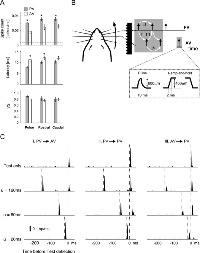
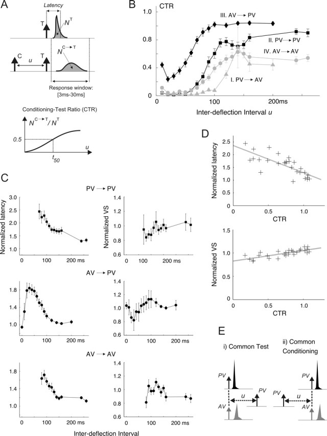
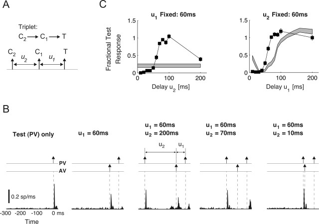
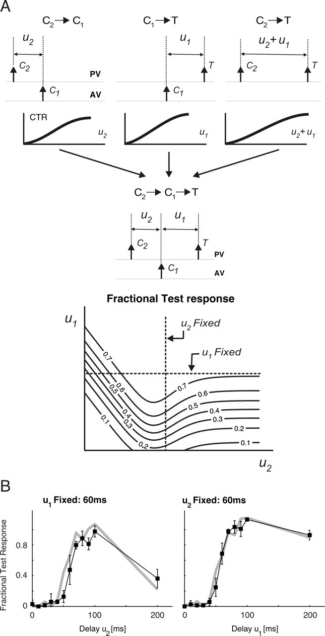
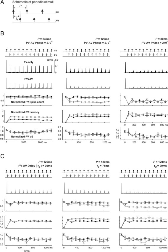
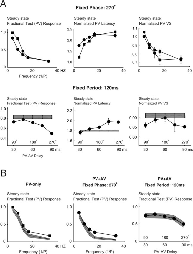
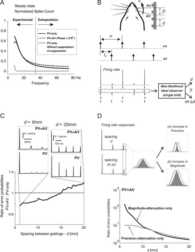
Spatiotemporal response integration across the neural receptive field (RF) is a general feature of sensory coding and has an important role in shaping responses to naturalistic stimuli. In the primary somatosensory cortex of the rat vibrissa pathway, such integration across the vibrissa array strongly shapes the coding of spatiotemporally distributed deflections. Using a spatiotemporal paired-pulse paradigm, this study revealed that fundamentally different types of pairwise interactions have similar qualitative behavior but that the magnitude, latency, and precision of the neural responses depend on the specific RF components being engaged. In all cases, however, increase in the suppression of response magnitude accompanied a lengthening of latency and a decrease in response precision. Furthermore, nonlinear interactions evoked by stimulation of multiple RF subregions strongly influence both response magnitude and timing to more complex sequences. Despite their complexity, such response interactions are highly predictable from elementary pairwise interactions. To understand the functional role of spatiotemporal interactions in coding, we developed a response model that incorporated the experimentally measured modulations in response magnitude, latency, and precision induced by cross-vibrissa interactions. Simulations of a simplified textural discrimination task indicate that spatiotemporal interactions enhance discrimination under certain stimulus time scales. This improvement follows from a nonlinear response property that acts to restore the neural response in the face of suppression. Together, the present findings highlight the role of response integration in shaping single-cell responses and provide predictions about how changes in response parameters influence coding accuracy.

Figure 1.

Pairwise interactions for a multi-vibrissa stimulus. A, From top to bottom, bar plots illustrate the averaged spike count, latency, and VS of isolated PV (gray bars) and AV (open bars) responses to the three types of stimuli used in this study. Error bars denote ±1 SEM. The asterisks mark the cases in which the difference between PV and AV measurements was significant (p < 0.05 in all cases; t test). B, Schematic of whisking geometry and evoked contact times for a PV–AV pair over a corrugated surface. White arrows and the corresponding labels I–IV identify four types of pairwise interactions that are experimentally measured here (I, PV→AV; II, PV→PV; III, AV→PV; IV, AV→AV). Additionally, the dashed box illustrates the amplitudes and time courses of both pulse and ramp-and-hold stimuli used in the study. C, Example of pairwise interactions for an individual cell. Each column shows the response to a particular pairwise sequence at three values of interdeflection delay u. In each column, the first row shows the first-order (baseline) deflection response. Rows 2–4 represent responses to deflection pairs with u = 160, 60, and 20 ms, respectively. All PSTHs are shown with time bins of 2 ms. Vertical dashed lines represent deflection times. The AV→AV interaction is not shown here because of its similarity to the PV→PV response for this cell; see Figure 2 for a summary of all pairwise responses (including AV→AV).

Figure 2.

The effects of pairwise interactions on the deflection response. A, The CTR was computed for a range of IDIs by (1) computing the spike-count response to the test (T) stimulus (N^C→T) in presence of a preceding conditioning (C) deflection and (2) normalizing this quantity by the response measured when T is presented in isolation (N^T). Spike count is computed as the area under the measured PSTHs over the 3–30 ms poststimulus time window. Latency represents the center of mass of the PSTH. VS quantifies the precision of the PSTH response and is defined in Materials and Methods (see Response measures). B, Average CTR measurements for pulse stimuli: I, PV→AV (gray triangles); II, PV→PV (black squares); III, AV→PV (black diamonds); IV, AV→AV (gray circles). Error bars represent 1 SEM, computed with n = 18. Qualitatively similar results were obtained using square-wave stimuli (n = 12). C, Both the latency and the VS of test responses in the presence of the conditioning stimulus are normalized to the values measured for the test presented in isolation. The resulting normalized latency (left column) and VS (right column) curves are shown for the PV→PV, AV→PV, and AV→AV interactions. The corresponding results for PV→AV are not shown because the majority of the estimates were unreliable as a result of the typically small AV responses (see text). D, The top scatter plot shows the relationship between the CTR value and the normalized latency of the PV response; PV→PV and AV→PV data are combined, so that each point on this plot corresponds to an average measurement at a given IDI. The x-coordinate of the point is the population-averaged (n = 18) CTR value at that IDI; its y-coordinate represents the corresponding population-averaged normalized latency. The gray line shows the linear regression of the latency ratio onto the CTR value (r = −0.76; p < 1e-4; y = −1.08x + 2.36). The bottom scatter plot illustrates an analogous relationship between the CTR value and the normalized test VS (r = 0.77; p < 1e-4; y = 0.23x + 0.83). E, Conditioning→test sequences are divided into two groups. i, Common test stimulus (left). For pulse stimuli, these consist of PV→PV and AV→PV. ii, Common conditioning stimulus (right), which for pulse stimuli considered here consist of PV→PV and PV→AV. A similar grouping can also be made using the AV→AV as the basis for comparison (in place of PV→PV).

Figure 3.

Nonlinear response interactions. A, Schematic of stimulus triplet. For the sequence C₂→C₁→T, the test response is measured under two scenarios. First, delay u₁ was fixed at 60 ms, and u₂ varied over the range 0–200 ms in 10 ms increments. Next, u₂ was fixed at 60 ms as u₁ varied over the same range. B, PSTH responses for the sequence C₂→C₁→T (specifically, PV→AV→PV) for different values of delay u₂. The leftmost plot shows the first-order test (PV) response. To its right, the response to the pairwise sequence AV→PV is shown (u₁ = 60 ms). The next three plots show the response to the third-order sequence PV→AV→PV as the delay u₁ was fixed at 60 ms, whereas u₂ equaled 200, 70, and 10 ms, respectively. C, The third-order normalized spike counts (fractional test response curves) for the cell shown in B are shown as functions of u₂ (left, ▪; u₁ = 60 ms) and of u₁ (right, ▪; u₂ = 60 ms). Error bars show ±1 SEM. The gray bands represent the corresponding measurements (and their associated uncertainties) for the second-order sequence C₁→T over the same delay range u₁ and u₂ (mean ± 1 SEM).

Figure 4.

Prediction of nonlinear interactions from constituent second-order effects. A, Schematic representing the constituent second-order interactions that combine to form the effective third-order fractional test response to the sequence C₂→C₁→T. The predicted response is a function of the two constituent delays u₁ and u₂ and is shown through a contour plot for an example case. B, Agreement between measured (black line with ▪) and predicted (gray line) Fractional test responses is shown for pulse stimuli, as functions of both u₂ (left) and u₁ (right). Error bars represent SEMs of the measured values. Over the population of cells, the coefficients of correlation between measured and predicted third-order responses of a single-cell were (mean ± SEM) 0.82 ± 0.03 for u₁ = 60 ms and 0.77 ± 0.05 for the u₂ = 60 ms case.

Figure 5.

Frequency and phase dependence of transient responses to periodic stimuli. A, Schematic of periodic stimuli. For PV-only cases, stimulation period P took five values: 240, 120, 80, 60, and 30 ms. For the two-vibrissa case, first the PV–AV phase delay was fixed at 270°, whereas the period ranged over the same values as above. Next, the stimulation period was fixed at 120 ms, whereas the PV–AV time delay t_d varied over the range 30–90 ms in 15 ms increments. B, Each column represents results from a distinct stimulation pattern (from left to right: 240, 120, and 80 ms). For each column, the top panel in each plot represents the periodic pulse deflections and the middle two panels show the average firing rate for all cells (n = 18) in response to PV-only and two-vibrissa (PV and AV) stimuli (top plot, PV-only response, black; bottom plot: response to PV and AV, gray). The next three panels show, respectively, the normalized spike counts, latencies, and VSs of PV responses evoked by single (black) and combined (gray) PV–AV deflections. Error bars represent ±1 SEM. C, Dependence of transient responses on the PV–AV time delay for a stimulation period of 120 ms. Results for t_d = 30, 75, and 90 ms are shown in the left, middle, and right columns, respectively. For each column, the order of the panels is the same as that described in B.

Figure 6.

Frequency and phase dependence of steady-state responses to periodic stimuli. A, The top row shows a comparison between three aspects of steady-state PV response (from left to right: spike count, latency, and VS) to single- and multi-vibrissa deflections as a function of frequency (PV-only, ▪; PV–AV with phase delay fixed at 270°, •). All measures represent averages over n = 18 cells, with error bars representing ±1 SEM. Similarly, the bottom row shows the corresponding measurements of PV responses as a function of the PV–AV time delay for a fixed stimulation period of 120 ms. The horizontal axes represent the PV–AV delay as both time (i.e., t_d, in millisecond) and phase (i.e., 360° × t_d/P). B, Predictability of steady-state responses for single- and multi-vibrissa periodic stimuli. From left to right, the plots consist of the following: (1) steady-state responses for PV-only stimuli as a function of frequency; (2) steady-state responses for paired-vibrissa stimuli as a function of frequency (phase is fixed at 270°); and (3) steady-state responses for paired-vibrissa stimuli as a function of varying PV–AV time-delay (period fixed at 120 ms). For each plot, the solid line represents the experimentally measured averaged response. The dashed lines represent the averaged predictions (for all cells). The gray areas are the regions of uncertainty (±1 SEM) for the predictions.

Figure 7.

Limits to discrimination performance for single- and two-vibrissa stimuli. A, Simulated normalized PV spike counts in response to PV-only (solid line) and paired-vibrissa (dashed line; PV–AV phase, 270°) stimuli; all simulations were based on the response model described in Results. The CTR curves used in simulations were obtained by parametrically fitting sigmoidal functions to population-averaged CTR curves. The gray curve shows the simulated PV-only response in the absence of suppression-of-suppression. The range of frequencies for which the response model was verified experimentally, along with the range over which the model was extrapolated are labeled as Experimental and Extrapolation, respectively. B, The whisking model generates idealized single- and paired-vibrissa pulse deflections characterized by their occurrence times. With simple geometrical considerations, the stimulation period P and the PV–AV time delay t_d are expressed as follows: P = d/v and t_d = (D mod d)/v, where d, v, and D represent the grating spacing, vibrissa-tip velocity, and inter-vibrissa separation, respectively. For a given geometry and the resulting deflection times, the model described in Materials and Methods generates a pair of firing-rate responses corresponding to surface gratings of d and d + Δd; an example of the firing rate and response rasters is shown. Next, an ideal observer matches the spiking response to the texture that most likely gave rise to that response. C, This plot shows, as a function of grating spacing, the ratio of P_error with two vibrissae to that obtained using only the PV. In all cases, Δd = 0.05 mm. Qualitatively similar results were obtained for other Δd values, although absolute performance improved with increasing Δd (data not shown). D, Changes in P_error as a result of spatiotemporal interactions are attributed to changes in response precision (a) and response magnitude (b). The firing rate responses evoked by spacings of d and d + Δd are shown on the left; the responses to a single stimulus cycle are considered in more detail. For a pair of equally likely surfaces, P_error based on single-trial observations (spikes) of a single response cycle scales with the extent of temporal overlap between the two firing rates; this overlap is shown by the shaded area. An increase in response precision reduces the temporal overlap between the pair of responses (a). In contrast, an increase in response magnitude (b) does not change the fractional overlap between the two responses. It lowers P_error by increasing the likelihood of observing one or more spikes in response: without spikes, P_error is at its maximum (i.e., one-half).

References

1. Ahissar E, Haidarliu S, Zacksenhouse M (1997). Decoding temporally encoded sensory input by cortical oscillations and thalamic phase comparators. Proc Natl Acad Sci USA 94:11633–11638. - PMC - PubMed
1. Ahissar E, Sosnik R, Haidarliu S (2000). Transformation from temporal to rate coding in a somatosensory thalamocortical pathway. Nature 406:302–306. - PubMed
1. Ahissar E, Sosnik R, Bagdasarian K, Haidarliu S (2001). Temporal frequency of whisker movement. II. Laminar organization of cortical representations. J Neurophysiol 86:354–367. - PubMed
1. Andermann ML, Ritt J, Neimark MA, Moore CI (2004). Neural correlates of vibrissa resonance: band-pass and somatotopic representation of high-frequency stimuli. Neuron 42:451–463. - PubMed
1. Arabzadeh E, Zorzin E, Diamond ME (2005). Neuronal encoding of texture in the whisker sensory pathway. PLoS Biol 3:0155–0165. - PMC - PubMed
Publication types
LinkOut - more resources