Weak pairwise correlations imply strongly correlated network states in a neural population

Abstract

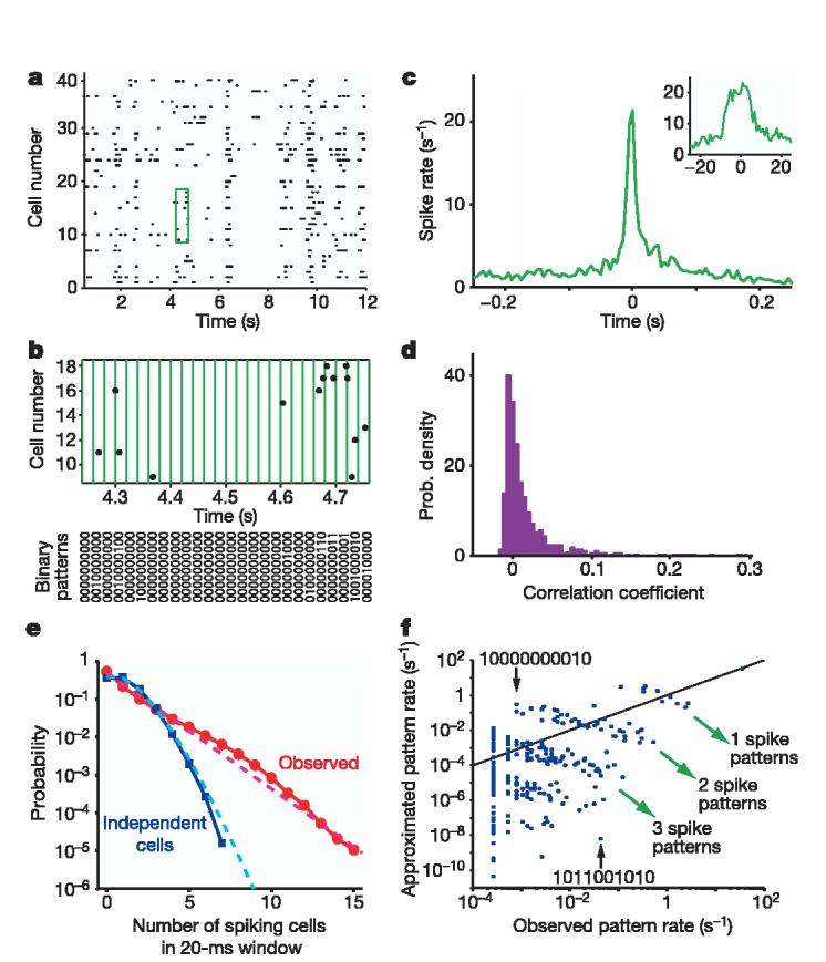
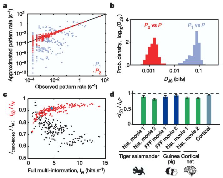
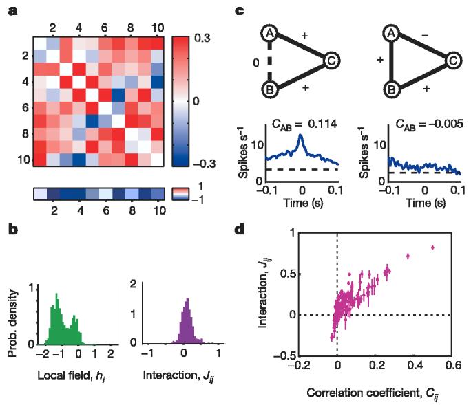
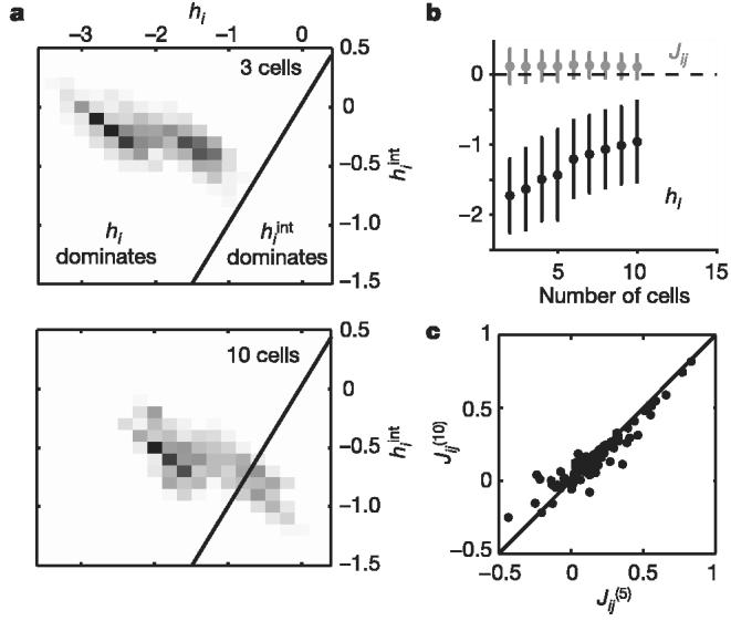
Biological networks have so many possible states that exhaustive sampling is impossible. Successful analysis thus depends on simplifying hypotheses, but experiments on many systems hint that complicated, higher-order interactions among large groups of elements have an important role. Here we show, in the vertebrate retina, that weak correlations between pairs of neurons coexist with strongly collective behaviour in the responses of ten or more neurons. We find that this collective behaviour is described quantitatively by models that capture the observed pairwise correlations but assume no higher-order interactions. These maximum entropy models are equivalent to Ising models, and predict that larger networks are completely dominated by correlation effects. This suggests that the neural code has associative or error-correcting properties, and we provide preliminary evidence for such behaviour. As a first test for the generality of these ideas, we show that similar results are obtained from networks of cultured cortical neurons.

Figure 1

Weak pairwise cross-correlations and the failure of the independent approximation. a, A segment of the simultaneous responses of 40 retinal ganglion cells in the salamander to a natural movie clip. Each dot represents the time of an action potential. b, Discretization of population spike trains into a binary pattern is shown for the green boxed area in a. Every string (bottom panel) describes the activity pattern of the cells at a given time point. For clarity, 10 out of 40 cells are shown. c, Example cross-correlogram between two neurons with strong correlations; the average firing rate of one cell is plotted relative to the time at which the other cell spikes. Inset shows the same cross-correlogram on an expanded time scale; x-axis, time (ms); y-axis, spike rate (s⁻¹). d, Histogram of correlation coefficients for all pairs of 40 cells from a. e, Probability distribution of synchronous spiking events in the 40 cell population in response to a long natural movie (red) approximates an exponential (dashed red). The distribution of synchronous events for the same 40 cells after shuffling each cell's spike train to eliminate all correlations (blue), compared to the Poisson distribution (dashed light blue). f, The rate of occurrence of each pattern predicted if all cells are independent is plotted against the measured rate. Each dot stands for one of the 2¹⁰ = 1,024 possible binary activity patterns for 10 cells. Black line shows equality. Two examples of extreme mis-estimation of the actual pattern rate by the independent model are highlighted (see the text).

Figure 2

A maximum entropy model including all pairwise interactions gives an excellent approximation of the full network correlation structure. a, Using the same group of 10 cells from Fig. 1, the rate of occurrence of each firing pattern predicted from the maximum entropy model P₂ that takes into account all pairwise correlations is plotted against the measured rate (red dots). The rates of commonly occurring patterns are predicted with better than 10% accuracy, and scatter between predictions and observations is confined largely to rare events for which the measurement of rates is itself uncertain. For comparison, the independent model P₁ is also plotted (from Fig. 1f; grey dots). Black line shows equality. b, Histogram of Jensen–Shannon divergences (see Methods) between the actual probability distribution of activity patterns in 10-cell groups and the models P₁ (grey) and P₂ (red); data from 250 groups. c, Fraction of full network correlation in 10-cell groups that is captured by the maximum entropy model of second order, I₍₂₎/I_N, plotted as a function of the full network correlation, measured by the multi-information I_N (red dots). The multi-information values are multiplied by 1/Δτ to give bin-independent units. Every dot stands for one group of 10 cells. The 10-cell group featured in a is shown as a light blue dot. For the same sets of 10 cells, the fraction of information of full network correlation that is captured by the conditional independence model, I_cond–indep/I_N, is shown in black (see the text). d, Average values of I₍₂₎/I_N from 250 groups of 10 cells. Results are shown for different movies (see Methods), for different species (see Methods), and for cultured cortical networks; error bars show standard errors of the mean. Similar results are obtained on changing N and Δτ; see Supplementary Information.

Figure 3

Pairwise interactions and individual cell biases, as in equation (1). a, Example of the pairwise interactions J_ij (above) and bias values (or local fields) h_i (below) for one group of 10 cells. b, Histograms of h_i and J_ij values from 250 different groups of 10 cells. c, Two examples of 3 cells within a group of 10. At left, cells A and B have almost no interaction (J_AB = −0.02), but cell C is very strongly interacting with both A and B (J_AC = 0.52, J_BC = 0.70), so that cells A and B exhibit strong correlation, as shown by their cross-correlogram (bottom panel). At right, a ‘frustrated’ triplet, in which cells A and B have a significant positive interaction (J_AB = 0.13), as do cells B and C (J_BC = 0.09), but A and C have a significant negative interaction (J_AC = −0.11). As a result, there is no clear correlation between cells A and B, as shown by their cross-correlogram (bottom panel). d, Interaction strength J_ij plotted against the correlation coefficient C_ij; each point shows the value for one cell pair averaged over many different groups of neighbouring cells (190 pairs from 250 groups), and error bars show standard deviations.

Figure 4

Interactions and local fields in networks of different size. a, Greyscale density map of the distribution of effective interaction fields experienced by a single cell $h_i^{\mathrm{int}}$ versus its own bias or local field h_i (see the text); distribution formed over network configurations at each point in time during a natural movie for n = 1,140 3-cell groups (top panel) and n = 250 10-cell groups (bottom panel). Black line shows the boundary between dominance of local fields versus interactions. b, Mean interactions J_ij and local fields h_i describing groups of N cells, with error bars showing standard deviations across multiple groups. c, Pairwise interaction in a network of 10 cells $J_{\mathit{ij}}^{\left(10\right)}$ plotted against the interaction values of the same pair in a sub-network containing only 5 cells $J_{\mathit{ij}}^{\left(5\right)}$. Line shows equality.

Figure 5

Extrapolation to larger networks. a, Average independent cell entropy S₁ and network multi-information I_N, multiplied by 1/Δτ to give bin-independent rates, versus number of cells in the network N. Theoretically, we expect I_N ∝ N(N − 1) for small N; the best fit is I_N ∝ N^1.98±0.04. Extrapolating (dashed line) defines a critical network size N_c, where I_N would be equal to S₁. b, Information that N cells provide about the activity of cell N + 1, plotted as a fraction of that cell's entropy, S(σ_i), versus network size N; each point is the average value for many different groups of cells. Extrapolation to larger networks (dashed line, slope = 1.017 ± 0.052) defines another critical network size N_c, where one would get perfect error-correction or prediction of the state of a single cell from the activity of the rest of the network. c, Examples of ‘check cells’, for which the probability of spiking is an almost perfectly linear encoding of the number of spikes generated by the other cells in the network. Cell numbers as in Fig. 1.

References

1. Hopfield JJ, Tank DW. Computing with neural circuits: a model. Science. 1986;233:625–633. - PubMed
1. Georgopoulos AP, Schwartz AB, Kettner RE. Neuronal population coding of movement direction. Science. 1986;233:1416–1419. - PubMed
1. Hartwell LH, Hopfield JJ, Leibler S, Murray AW. From molecular to modular cell biology. Nature. 1999;402(Suppl C):47–52. - PubMed
1. Barabási A-L, Oltvai ZN. Network biology: Understanding the cell's functional organization. Nature Rev. Genet. 2004;5:101–113. - PubMed
1. Perkel DH, Bullock TH. Neural coding. Neurosci. Res. Prog. Sum. 1968;3:221–348.
Publication types