

Review
doi: 10.1021/cr0404343.
Single-molecule fluorescence studies of protein folding and conformational dynamics
Affiliations
- PMID: 16683755
- PMCID: PMC2569857
- DOI: 10.1021/cr0404343
Item in Clipboard
Review
Single-molecule fluorescence studies of protein folding and conformational dynamics
Chem Rev.
2006 May.
No abstract available
Figures
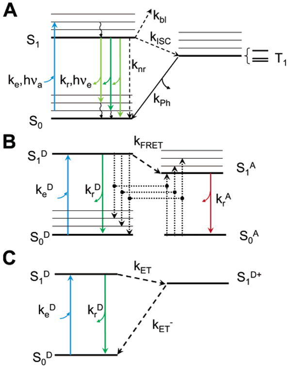
Jablonski diagrams for fluorescence, FRET and ET. (A) Upon absorption of a photon of energy hνa close to the resonance energy ES1 – ES0, a molecule in a vibronic sublevel of the ground singlet state S0 is promoted to a vibronic sublevel of the lowest excited singlet state S1. Nonradiative, fast relaxation brings the molecule down to the lowest S1 sublevel in picoseconds. Emission of a photon of energy hνe < hνa (radiative rate kr) can take place within nanoseconds and bring back the molecule to one of the vibronic sublevels of the ground state. Alternatively, collisional quenching may bring the molecule back to its ground state without photon emission (nonradiative rate knr). A third type of process present in organic dye molecules is ISC to the first excited triplet state T1 (rate kISC). Relaxation from this excited state back to the ground state is spin-forbidden, and thus, the lifetime of this state (1/kPh) is in the order of microseconds to milliseconds. Relaxation to the ground state takes place by either photon emission (phosphorescence) or nonradiative relaxation. (B) FRET involves two molecules: a donor D and an acceptor A whose absorption spectrum overlaps the emission spectrum of the donor. Excitation of the acceptor to the lowest singlet excited state is a process identical to that described for single-molecule fluorescence (A). In the presence of a nearby acceptor molecule (within a few nanometers), donor fluorescence emission is largely quenched by energy transfer to the acceptor by dipole–dipole interaction with a rate kFRET ∼ R−6, where R is the D–A distance. The acceptor and donor exhibit fluorescent emission following the rules outlined in part A and omitted in this diagram for simplicity. (C) PET effectively oxidizes the donor molecule with a rate kET ∼ exp (–βR), preventing its radiative relaxation. Upon reduction, the molecule relaxes nonradiatively to its ground state. In this scheme, the electron acceptor does not fluoresce and is therefore not represented.
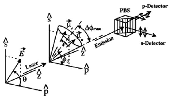
Polarization spectroscopy geometry. E⃗ is the electric field, making an angle θ with the p polarization axis. The excitation propagates along axis z, which is also the collection axis. μ⃗a and μ⃗e are the absorption and emission dipole moments, initially aligned. ν represents the rotational diffusion of the emission dipole during the excited lifetime. The dipole is supposed to be confined in a cone positioned at an angle φ0 projected on the (s, p) plane and having a half-angle Δφmax. A polarizing beam splitter splits the collected emission in two signals Is and Ip, which are simultaneously recorded by APDs. Adapted Figure 1 with permission from ref 223 (http://link.aps.org/abstract/PRL/v80/p2093 ). Copyright 1998 by the American Physical Society.
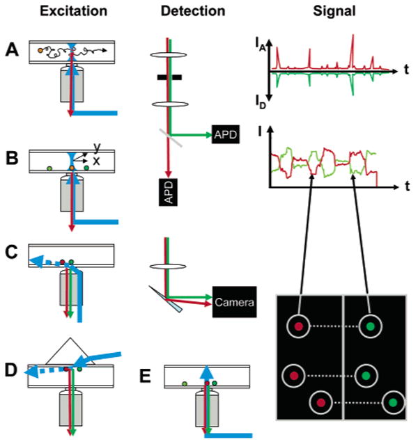
Experimental geometries in single-molecule fluorescence spectroscopy. Two main types of geometries can be used for single-molecule fluorescence spectroscopy: confocal and wide field. In the confocal geometry (A, B), a collimated laser beam is sent into the back focal plane of a high numerical aperture objective lens, which focuses the excitation light into a diffraction limited volume (or point spread function, PSF) in the sample. PSF engineering can be used at this stage to shape the excitation volume in order to gain resolution in any dimension. Fluorescence emitted by molecules present in this volume is collected by the same objective and transmitted through dichroic mirrors, lenses, and color filters to one or several point detectors (APD). An important aspect of this geometry is the presence of a pinhole in the detection path, whose size is chosen such as to let only light originating from the region of the excitation PSF reach the detectors. Freely diffusing molecules (A) will yield signals comprised of bursts of various size and duration (but typically less than a few milliseconds), as indicated schematically on the RHS. Immobile molecules (B) will need to be first localized using a scanning device (indicated as two perpendicular arrows x and y), before recording can commence. Typical time traces are comprised of one or more fluctuating intensity levels until the molecule eventually bleaches after a few seconds, as indicated schematically on the RHS. The wide-field geometry (C–E) can be used in two different modes: (C, D) TIR or (E) epifluorescence. In TIR, a laser beam is shaped in such a way that a collimated beam reaches the glass–buffer interface at a critical angle θ = sin−1(nbuffer/nglass), where n designates the index of refraction. This creates an evanescent wave (decay length of a few hundreds of nanometers) in the sample (dashed arrow), which only excites the fluorescence of the molecules in the vicinity of the surface, resulting in a very low background. TIR can be obtained either with illumination through the objective (C) or by coupling the laser through a prism (D); both methods have their advantages and inconveniences (for details, see ref 224). In epifluorescence (E), a laser beam focused at the back focal plane of the objective or a standard arc lamp source is used to illuminate the whole sample depth, possibly generating additional background signals. A wide-field detector (camera) is used in all three cases, allowing the recording of several single-molecule signals in parallel, although with a potentially smaller time resolution than that achieved with point detectors. The image on the RHS represents the case of a dual-color experiment, where both spectral channels are imaged simultaneously on the same camera (signals from the same molecule are connected by dotted line). Individual intensity trajectories can be extracted from movies, resulting in similar information as that obtained with the confocal geometry.
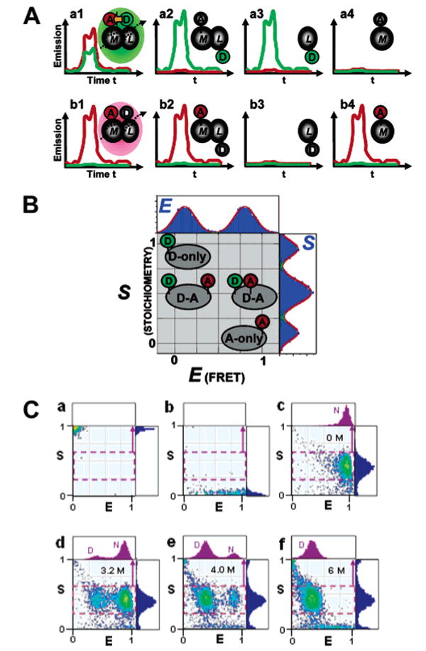
Fluorescence-aided molecular sorting using μs-ALEX. ALEX allows detection of D excitation- and A excitation-based fluorescence emission for single diffusing molecules, enabling fluorescence-aided molecular sorting. The advantages of ALEX over traditional single-laser excitation is exemplified in part A, using the interaction between a D-labeled ligand (L) and an A-labeled macromolecule as an example (D and A depicted as green and red ovals, respectively). The top panel shows emission caused by D-excitation using single-laser excitation. Short distances within the M–L complex cause emission predominantly in the acceptor channel (red curves), whereas large distances mainly result in D emission. Note that there is no discrimination between a low-FRET complex and the fluorescence emission signature resulting from unbound L, and free M is not detectable. ALEX allows direct excitation of the A, allowing one to distinguish between low-FRET complexes and unbound acceptor. (B) Two-dimensional E–S histogram for single-molecule sorting. The conventional FRET efficiency E sorts species according to D–A distance and thus reports on structure. The novel stoichiometric ratio S reports on D/A stoichiometry. The additional dimension allows D-only and A-only species to be distinguished from low- and high-FRET subpopulations, respectively. (C) ALEX-based probing of the equilibrium unfolding of CI2, specifically labeled with Alexa647 at the N terminus and Alexa488 at position 40. Representative 2D E–S histograms of D-only-labeled CI2 (a), A-only-labeled CI2 (b) and D/A-labeled CI2 at various concentrations of GdmCl (c–f). One-dimensional histograms of the stoichometric ratio S are shown in blue color to the right of each histogram. One-dimensional histograms of the FRET efficiency E for each sample are displayed on top of each 2D histogram in purple. See the text for details. Parts A and B are adapted with permission from ref 111. Copyright 2004 National Academy of Sciences U.S.A. Part C is reprinted with permission from ref 173. Copyright 2005 Cold Spring Harbor Laboratory Press.
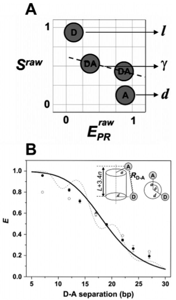
Application of μs-ALEX for accurate FRET measurements in biomolecules at the single-molecule level. (A) Species required for recovering all correction factors needed for accurate ratiometric E measurements. D-only species provide the D leakage factor l, A-only species provide the A direct excitation factor d, and two D–A species with a large difference in E provide the correction factor γ. (B) Comparison of E values measured for DNA fragments with values predicted from cylindrical models of DNA. ALEX-based E values (filled black dots) and E values from ensemble measurements (open circles) are shown. The solid black curve represents the theoretical dependence of the E value on D–A separation with the D probe proximal to the DNA helical axis, while the dotted line represents theoretical E values with the D probe distal from the DNA helical axis. Note that in all cases, a single-molecule-based E value fit better to theoretical values than ensemble-based values. Adapted with permission from ref 119. Copyright 2005 Biophysical Society.
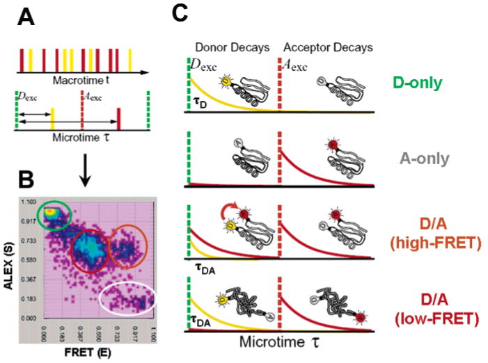
Principle of ns-ALEX. (A) Interlacing pulses from two lasers, Dexc (green, excites D) and Aexc (red, excited A), with a fixed delay between the detected photons; the Dexc laser pulse is measured with ∼500 ps resolution, providing information about fluorescence lifetime and the ability to classify photons according to Dexc or Aexc (i.e., whether time delay τ is before or after the Aexc pulse). (B) Two-dimensional E–S photon burst histogram resulting from single molecules of D/A-labeled CI2 diffusing through the laser focal spot in the presence of 4 M GdmCl. Values for the FRET efficiency E and stoichiometry ratio S are calculated and placed in a 2D E–S histogram. Four species are detected as follows: D only (green circle), A only (grey circle), folded CI2 (high-FRET) (orange circle), and denatured CI2 (low-FRET) (red circle). The corresponding time-resolved fluorescence decay curves are extracted from the relevant portions of the photon stream and are depicted in part C. D-only molecules emit only after D excitation (yellow curve, leakage into the A channel removed for clarity), while A-only molecules only emit after A excitation (red trace). Unfolded proteins labeled with D and A emit D and A fluorescence after a Dexc pulse (ratio of intensities and lifetimes depend on FRET efficiency) and emit A fluorescence after Aexc. Folded proteins labeled with D and A emit similarly, except with a higher relative intensity of A as compared to D after the D excitation pulse and with a shorter D lifetime, indicating a higher FRET efficiency due to shorter average distance.
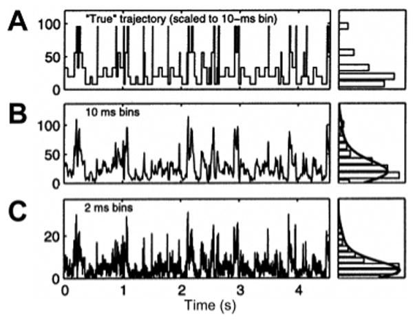
Time trace of a multistate single-molecule observable (photon counts). (A) Exact sequence of transition between states displayed with a time resolution allowing each transition to be readily observable. The histogram of intensity levels represented on the RHS exhibits five distinct states. (B) Real signal simulated by adding shot noise to the previous trace. Although indication of several levels is apparent from the various peak heights, the histogram on the RHS renders their indentification impossible. (C) Increasing the time resolution of the time trace 5-fold does not improve the situation, as shot noise becomes proportionally more important. Adapted with permission from ref 145. Copyright 2005 American Chemical Society.
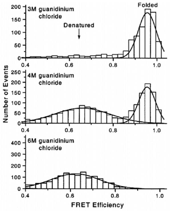
FRET efficiency distributions of CI2 at three different denaturant concentrations. Top, 3 M GdmCl (native conditions); middle, 4 M GdmCl (close to the midpoint of unfolding); and bottom, 6 M GdmCl (strongly denaturing conditions). The bimodal distribution of the FRET efficiency clearly indicates the two-state nature of the unfolding process. Adapted with permission from ref 110. Copyright 2000 National Academy of Sciences U.S.A.
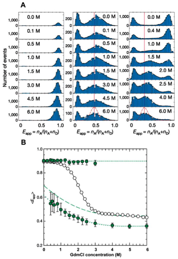
Probing the equilibrium unfolding of Csp with freely diffusing molecules. (A) FRET efficiency histograms for Pro6 (left), Pro20 (middle), and Csp (right) at various concentrations of denaturant. Black curves represent best fits of the experimental data to log-normal or Gaussian functions. The dashed line reflects the contribution of shot noise to the width of the distribution. (B) Dependence of the means of the measured FRET efficiency of Csp. Upper full symbols are derived from the native subpopulations, while lower full symbols are calculated from the denatured subpopulation. Open symbols are the apparent FRET efficiencies measured in an ensemble FRET experiment. The shift in the mean E of the denatured subpopulation of Csp most likely reflects a collapse of the polypeptide chain upon transfer from a good solvent (high concentrations of denaturant) to a poor solvent (low concentrations of denaturant). No such shift is seen in the folded subpopulation or in the rigid polyproline distance rulers. Note that the width of the distribution of the rigid polyproline rulers is comparable to the width of the denatured subpopulation of Csp, suggesting that slow conformational fluctuations on a time scale comparable or slower than the experiment (<1 ms). Adapted with permission from Nature (http://www.nature.com ), ref 70. Copyright 2002 Nature Publishing Group.
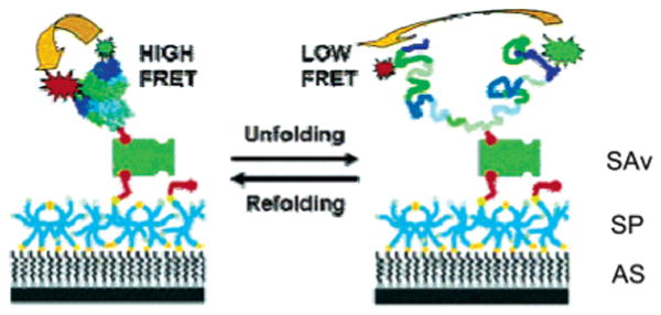
Schematic of protein immobilization on inert, biofunctionalized surfaces. Amino-silyated glass is coated with a layer of cross-linked six-arm SPs. Biotinylated and FRET pair-labeled RNAse H is added and coupled to the surface via biotin–SAv sandwich chemistry. Addition of denaturant destabilizes RNAse H, resulting in the population of denatured conformers. The interconversion between the folded and the denatured states can be followed using FRET between the donor and the acceptor fluorophores as a reaction coordinate. Adapted with permisison from ref 171. Copyright 2004 American Chemical Society.
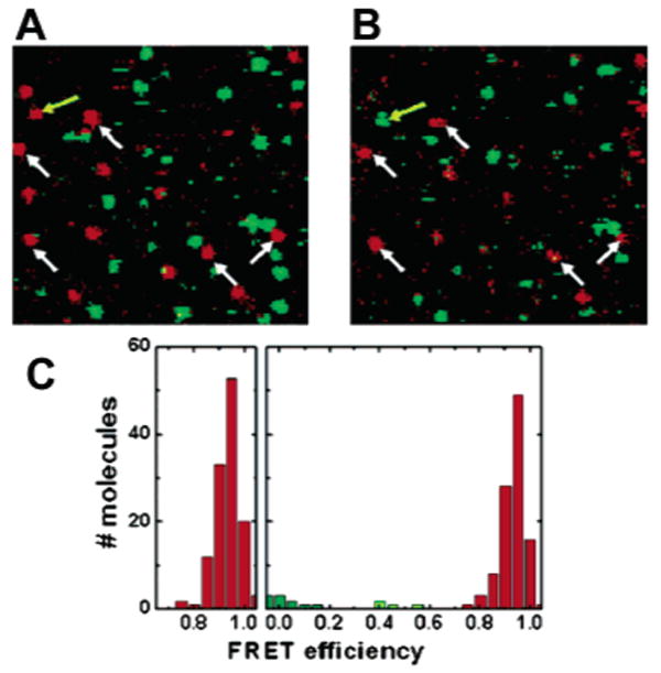
Confocal scans of a 10 μm × 10 μm sized area before (A) and after (B) 50 consecutive cyles of folding and unfolding. The white arrows indicate molecules that can be followed over many cycles. Out of >100 molecules, only four become trapped in a non-native conformation (one example is highlighted by a yellow arrow), demonstrating the high repellence of the polymer coating. (C) FRET histogram of >100 molecules before and after the folding–unfolding cycle. No increase in the width of the folded distribution is observable, ruling out structural heterogeneity induced by non-native interactions of the immobilized protein with the coated surface. Adapted with permission from ref 170. Copyright 2004 Wiley-VCH Verlag GmbH.
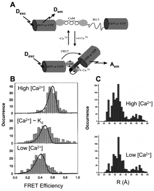
FRET study of CaM. (A) Schematic structures of the cameleon molecules used in ref 184. The GFPs are drawn as rigid cylinders, reflecting their crystal structures. Schematic structures of CaM without Ca2+, disordered unbound 73, and of the Ca2+–CaM–73 complex. (B) Histograms of Förster energy transfer efficiency, deduced from single-copy measurements of cameleon molecules for three different concentrations of calcium: Ca2+ saturation, intermediate concentration, and calcium-free agarose gel. The solid lines are the expected energy transfer efficiency distribution from the experimental noise, including shot noise and background noise as explained in the text. (C) Distributions of CaM donor–acceptor distances at high and low calcium levels using 75 μs bins. Bins containing donor or acceptor counts that were eight times above the standard deviation of the background signal, or six times above the standard deviation of the average sum of donor and acceptor counts, were included. (A) Adapted with permission from Nature (http://www.nature.com ), ref 187. Copyright 1997 Nature Publishing Group. (B) Reprinted with permission from ref 184. Copyright 2000 American Chemical Society. (C) Adapted with permission from ref 185. Copyright 2004 American Chemical Society.
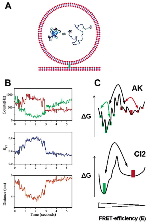
Probing conformational dynamics within single, surface-immobilized molecules. (A) Encapsulation of single molecules in lipid vesicles. Immobilization of the trapped molecule is achieved indirectly by tethering the biotinylated vesicle to a streptavidin-coated polymer coating. As the diameter of the encapsulating vesicle (∼100 nm) is considerably larger than the diameter of the trapped molecule, the trapped molecule can diffuse freely, thus minimizing a perturbation of the energy landscape due to confinement and nonproductive interactions of the trapped protein with the vesicle interior. (B) Representative single-molecule folding trajectories of encapsulated AK at denaturant concentrations around the midpoint of unfolding, conditions at which the native and denatured subpopulations are equally populated. The top panel shows time traces of the D and A emission (green and red, respectively), employing 20 ms bin times. D and A emission are anticorrelated, indicative of conformational transitions within the polypeptide. Notice, however, that the D emission continues to increase after bleaching of the acceptor (t ∼ 3 s), suggesting a variable environment (e.g., diffusion within the vesicle). Two types of fluctuations are visible in the E trajectory: fast, stepwise fluctuations that cannot be resolved and slow, continuous transitions that can take >1 s for completion. The middle panel depicts a FRET efficiency trajectory calculated from the signals in the top panel, whereas the interprobe distance trajectory (calculated according to Förster theory) is shown in the bottom panel. (C) Schematic of a 1D energy landscape for AK and CI2 at denaturant concentrations close to the midpoint of folding, obtained by averaging of the folding landscape over many degrees of freedom and projection onto the FRET efficiency axis. Both energy landscapes exhibit two global free energy minima separated by a free energy barrier, as suggested by the bimodal FRET efficiency distributions. The landscape of AK is characterized by local free energy barriers and traps, resulting in fluorescence time trajectories that can start and end at any FRET efficiency value (the population weight of the folded species is indicated by green bars, while the unfolded conformers are color-coded red). The landscape of CI2 is smoother, and time trajectories exhibit fluctuation between two relatively constant levels of FRET efficiencies. (A) Adapted with permission from ref 188. Copyright 2004 American Chemical Society. (B) Adapted with permission from ref 138. Copyright 2003 National Academy of Sciences USA.
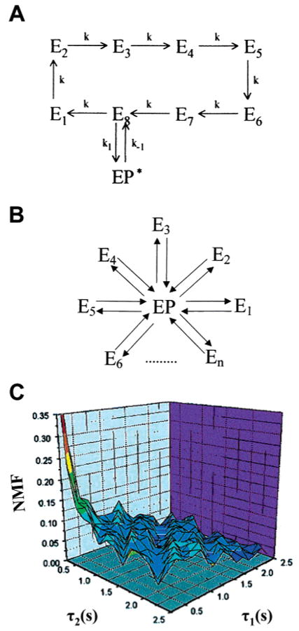
Single-molecule spectroscopy of HRP. Descriptions of two possible origins of the stretched exponential kinetics in the one-time autocorrelation of the fluorescence intensity observed in individual HRP enzymes. In part A, there are a number of intermediate states (Ek, k = 1,2,3,…,n) that the enzyme may traverse before a new product is formed (EP*). In part B, transitions to the EP state are exponential for each substrate turnover; however, each turnover may occur via any of the n channels, each with a different state transition probability. (C) Typical memory landscape NMF-(τ1,τ2) of a molecule observed for 110 s, showing that scheme A is appropriate for the description of the observed dynamic disorder in HRP. Adapted with permission from ref 199. Copyright 2000 National Academy of Sciences U.S.A.
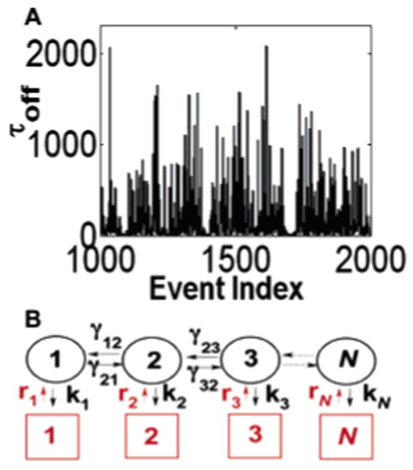
CALB enzyme activity. (A) The trajectory of the time durations of the off-state events as a function of chronological event index for a substrate concentration of 1.4 μM. Noticeable along this trajectory are groups of successive fast events (each event in the group has an off value of <35 ms). (B) The fluctuating enzyme model. The off state consists of a spectrum of N-coupled substates (circles). Also indicated are the coupling rates between the conformations and the enzymatic reaction rates. Squares indicate the on states. Reprinted with permission from ref 201. Copyright 2005 National Academy of Sciences U.S.A.
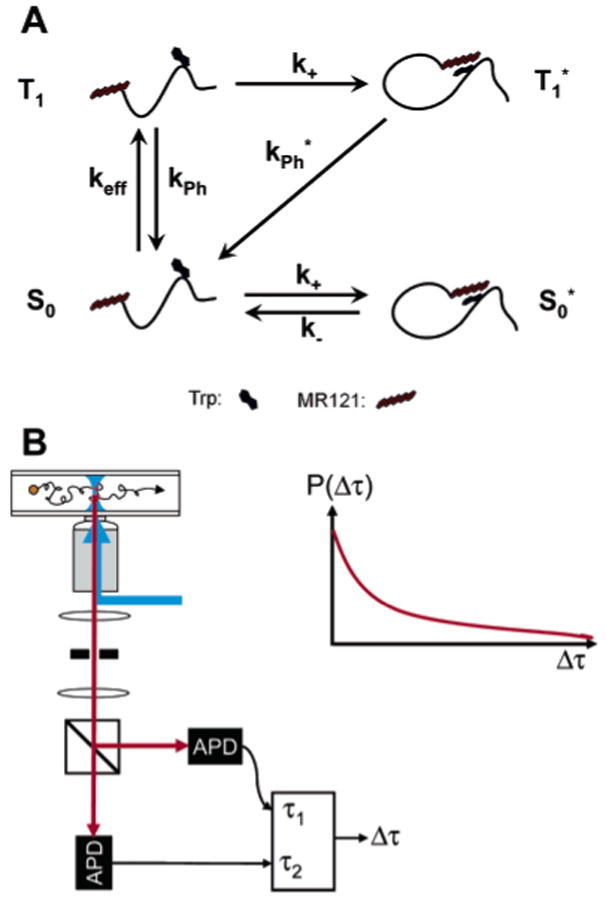
Peptide fluctuation dynamics studied by ET. (A) The dye/Trp association and subsequent efficient fluorescence quenching are used to reveal contact formation rate constants. keff, effective excitation rate in the triplet state; keff = kekISC/(kr + kISC), where ke, kr, and kISC are defined in Figure 1A; k+, association rate; k−, dissociation rate in the ground state; and kPh*, compound decay rate from the radical anion state T1* to S0 directly or via S0*. (B) Confocal detection setup used for PDD analysis. The emitted fluorescence is split by a polarizing beam splitter and collected by two APDs. The TTL pulses of each APD are recorded by TCSPC electronics, which measures the time delay between two successive photons, Δτ. The histogram of Δτ values constitutes the PDD. Adapted with permission from ref 94. Copyright 2003 American Chemical Society.
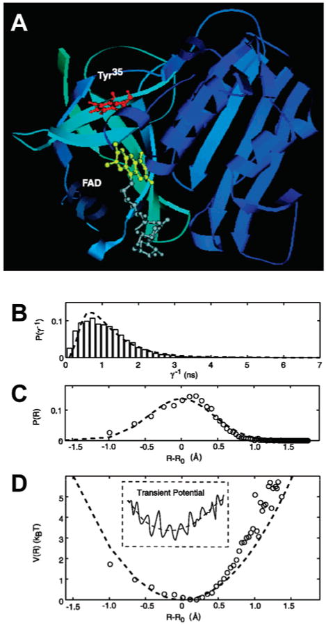
Enzyme conformational dynamics probes by ET. (A) Representative structure of the Fre/FAD complex from MD simulation. The fluorescent isoalloxazine moiety of FAD (yellow) sits in its binding pocket, in close proximity to the tyrosine residue (Tyr35), which dominates the quenching of flavin fluorescence in Fre. (B) Distribution of fluorescence lifetimes obtained from a single-molecule time trace. (C) Distribution of the FAD–Tyr35 edge-to-edge distance derived from the distribution in part B using β = 1.4 Å−1 in eq 14. (D) Potential of mean force calculated from part C. The dashed lines in all graphs correspond to fits to a harmonic potential of mean force around a center value R0, and variance θ = 0.19 Å2. Inset: Sketch of a transient rugged potential for the protein conformational motion projected to the experimentally accessible coordinate R. Adapted with permission from Science (http://www.aaas.org ), ref 31. Copyright 2003 American Association for the Advancement of Science.
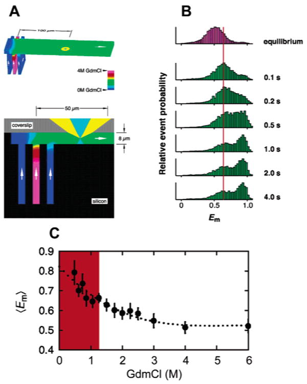
Probing single-molecule protein folding kinetics under nonequilibrium conditions. (A) Top: View of the mixing region of the microfluidic laminar mixing device, with the denaturant concentration indicated by a false color code. The laser beam (light blue) and collected fluorescence (yellow) are shown 100 μm from the center inlet. Bottom: Cross-section of the mixing region. (B) Histograms of measured FRET efficiency as a function of the mixing time. Within the first 100 ms of mixing, the expanded chain collapsed into a more compact coil structure, indicated by the slight increase in mean E. The collapsed denatured species reconfigure into the compact folded state on a time scale of a few seconds. Note that the mean E of the collapsed denatured subpopulation does not vary with time (red line) nor final denaturant concentration (data not shown). (C) Dependence of the mean E values of the collapsed coil state as a function of final denaturant concentration in the refolding buffer. The colored region highlights the denaturant range within which mean E values and distribution widths cannot be determined accurately using freely diffusing molecules under equilibrium conditions. Adapted with permission from Science (http://www.aaas.org ), ref 168. Copyright 2003 American Association for the Advancement of Science.
References
-
- Basché T, Moerner WE, Orrit M, Wild UP, editors. Single-Molecule Optical Detection, Imaging and Spectroscopy. VCH; Weinheim: 1997.
-
- Nie S, Zare RN. Annu Rev Biophys Biomol Struct. 1997;26:567. - PubMed
-
- Xie XS, Trautman JK. Annu Rev Phys Chem. 1998;49:441. - PubMed
-
- Moerner WE, Orrit M. Science. 1999;283:1670. - PubMed
-
- Weiss S. Science. 1999;283:1676. - PubMed
Publication types
MeSH terms
Substances
Grants and funding
LinkOut - more resources
Full Text Sources
Other Literature Sources
