Co-contraction and passive forces facilitate load compensation of aimed limb movements

Abstract

Vertebrates and arthropods are both capable of load compensation during aimed limb movements, such as reaching and grooming. We measured the kinematics and activity of individual motoneurons in loaded and unloaded leg movements in an insect. To evaluate the role of active and passive musculoskeletal properties in aiming and load compensation, we used a neuromechanical model of the femur-tibia joint that transformed measured extensor and flexor motoneuron spikes into joint kinematics. The model comprises three steps: first, an activation dynamics module that determines the time course of isometric force; second, a pair of antagonistic muscle models that determine the joint torque; and third, a forward dynamics simulation that calculates the movement of the limb. The muscles were modeled in five variants, differing in the presence or absence of force-length-velocity characteristics of the contractile element, a parallel passive elastic element, and passive joint damping. Each variant was optimized to yield the best simulation of measured behavior. Passive muscle force and viscous joint damping were sufficient and necessary to simulate the observed movements. Elastic or damping properties of the active contractile element could not replace passive elements. Passive elastic forces were similar in magnitude to active forces caused by muscle contraction, generating substantial joint stiffness. Antagonistic muscles co-contract, although there was no motoneuronal coactivation, because of slow dynamics of muscle activation. We quantified how co-contraction simplified load compensation by demonstrating that a small variation of the motoneuronal input caused a large change in joint torque.

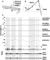
Figure 1.

Experimental setup and example of locust scratching behavior. A, The locust was tethered with its hindleg standing on a support (black square), which determined the start posture. Stimulation at either an anterior or a posterior location on the wing (triangles) initiated a scratching movement. The hindleg performed a targeted movement in which the end of the tibia was aimed at the stimulus location, followed by a cyclical component (trajectory shown as a black line for a scratch aimed at the posterior target). In half of the trials, a load was placed at the end of the tibia (circle). A three-dimensional optical motion capture system analyzed the locations of six reflective markers (crosses) and thus measured five joint angles (B) in each video frame. Joint angles φ and ψ were 0 when the leg was in a plane parallel to the sagittal body plane. C, Synchronous electromyograms were recorded of extensor (top channel, slow extensor tibiae, SETi) and flexor (bottom channels, proximal flexor, distal flexor) motor activity. Gray shading marks extensor burst activity.

Figure 2.

Scheme of the biomechanical model used to simulate locust scratching movements. Numbers indicate the order in which the components of the model were included, thus increasing its complexity in steps. The neuronal input consisted of slow motoneuron action potentials (SETi and slow flexor), which were transformed into the active state of the muscle using activation dynamics. The active state was scaled by the maximal possible isometric force and modified by passive elasticity, force–velocity, and force–length properties of the muscle. Muscle force was transformed into FT joint torque by moment arms given by the joint geometry. A joint damping component reduced the torque, depending on joint velocity. Tibial movement was calculated from joint torque using a forward dynamics algorithm. Co-contraction occurs when both antagonistic muscle models produce a nonzero torque.

Figure 3.

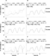
Typical recorded (dotted line) and simulated (solid line) FT joint angle time courses for different model variants, all of which included at least active isometric extensor and flexor force. The example movement was aimed at a posterior stimulus and had a loaded tibia. Top rows in each graph show the times of recorded slow motoneuron spikes (from top to bottom: SETi, slow proximal flexor, slow distal flexor). A, The simulation result with a PD component (RMSE of 29.6°). B, The time course for a model including PD and PE (RMSE of 6.1°). C, The time course including an additional force–velocity–property (RMSE of 7.0°). D, An additional force–length property (RMSE of 9.1°). In E, the PE was removed from the model variant including all other properties (RMSE of 28.4°). The small oscillations at second 1 and 2 are a simulation artifact, because the tibia moved against the physiological joint angle range constraint. In F, the PD was removed from the model with all properties (RMSE of 11.1°).

Figure 4.

RMSE for different muscle model variants (increasing from left to right), divided into 40 unloaded (open boxes) and 40 loaded (gray boxes) trials for five animals. Boxes show the lower and upper quartile, and whiskers represent 1.5 times the interquartile range. Using only extensor and flexor forces resulted in oscillatory movements and therefore created the largest RMSE of all models (column “force”). PD reduced the error, but a PE component decreased the error further, because it returned the tibia from extreme positions to the resting position. Addition of a force–velocity (FV) and force–length (FL) property did not reduce the error.

Figure 5.

Parameter distributions for the complete muscle model as used in variant 5 (solid lines, median; shadowed areas, 10,90 percentiles). A, Passive joint damping, which is proportional to joint velocity. B, Passive elasticity parabola for the musculotendon system. C, Force–velocity property of the muscle (negative velocities correspond to contracting muscle). The x-axes for the joint and muscle velocity graphs are scaled to maximal velocities observed in scratching behavior. D, Force–length property of the muscle.

Figure 6.

Generalization and parameter sensitivity of optimized muscle model variants. Generalization (white boxes), The RMSE for each trial was computed using a muscle model determined by mean values from all other trials from one animal. Generalization performance was best for a muscle model that included passive properties and the force–velocity property. Parameter sensitivity (gray boxes), Same error measure as in generalization test but using the extreme values of the optimized parameter ranges to illustrate sensitivity to parameter variation. Sensitivity was largest for passive damping and elasticity in model variants 2 and 3. Only in these cases were errors significantly larger than in the generalization test. Inset, The sample trajectory (RMSE of 13.0°) was generated using the average optimum of model variant 3 with passive damping and passive elasticity, which was the best model for individually optimized trials.

Figure 7.

Two sample trials (Ai, Aii, unloaded tibia; Bi, Bii, loaded tibia) with the net torque (bold solid line in Aii, Bii) decomposed into the separate torques generated by the extensor (top thin line) and flexor (bottom thin line) muscles, respectively. The bold dotted line shows the torque attributable to passive joint damping. The simulated time courses of the FT joint angle are shown in Ai and Bi. Because of co-contraction of both muscles and joint damping, the net torque in the unloaded trial is 28-fold lower than the average muscle-produced torque and thus was near the 0 axis. In the loaded trial, net torque is only 1.8-fold lower.

Figure 8.

Passive elasticity of antagonistic muscles depending on the FT joint angle. Although the passive force is modeled as a cubic parabola depending on muscle length, because of the moment arms, the resulting torque resembles a linear torque spring with respect to the joint angle. Its maximum absolute torques reach 54 μNm in the model.

Figure 9.

Active and passive components of torque production for all trials separated by stimulus position, loading condition (0, unloaded; L, loaded), and tibial movement direction for model variant 5. The relationship between passive and active torques strongly depends on the stimulus position. In anterior stimulus position, extensor torque is mostly generated passively (gray bars), because the tibia is likely in a flexed position. In contrast, flexor generated torques are mostly active (black bars). For posterior movements, the leg is more extended than in anterior movements; therefore, the extensor passive torque contributes less to total torque, whereas the flexor passive torque is larger than for anterior movements. Net torque (white asterisks, extensor torque minus flexor torque and damping) is mostly positive to compensate gravity.

Figure 10.

Active extensor torque (black boxes) and passive extensor torque (gray boxes) for n = 90 extensions with a minimum mean joint velocity of 100°/s and a duration of minimally 160 ms. In the first half of an extension, passive torques were larger than actively generated torques.

Figure 11.

Femur–tibia joint torque during extensions is the extensor active and passive torque (left bar of each pair) minus flexor torque and damping (right bar of each pair). In unloaded trials (gray bars), co-contraction of both muscles resulted in a median net torque of 1.1 μNm, although each of the muscles produces >25 μNm. In loaded trials (black bars), extensor torque is increased by 45.8% and flexor torque is reduced by 20.9%, which results in a 16-fold increase of net torque to 18.4 μNm.

Figure 12.

Measured probability for an SETi spike (black bars) or a slow flexor tibiae motoneuron spike (gray bars) defined by the ratio between the number of spikes and the number of recorded FT joint angles in each bin. The probability for an SETi spike increased for increasing joint angles, whereas the probability for a slow flexor spike decreased for increasing joint angles.

References

1. Ahn A, Full R (2002). A motor and a brake: two leg extensor muscles acting at the same joint manage energy differently in a running insect. J Exp Biol 205:379–389. - PubMed
1. Bässler U, Stein W (1996). Contributions of structure and innervation pattern of the stick insect extensor tibiae muscle to the filter characteristics of the muscle-joint system. J Exp Biol 199:2185–2198. - PubMed
1. Bennet-Clark H (1975). The energetics of the jump of the locust Schistocerca gregaria. J Exp Biol 63:53–83. - PubMed
1. Berkowitz A, Laurent G (1996). Local control of leg movements and motor patterns during grooming in locusts. J Neurosci 16:8067–8078. - PMC - PubMed
1. Blackburn L (2005). Behavioural and physiological differences in the motor systems of solitarious and gregarious locusts. PhD thesis University of Cambridge.
Publication types
LinkOut - more resources