Statistics of knots, geometry of conformations, and evolution of proteins

Abstract

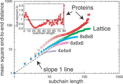
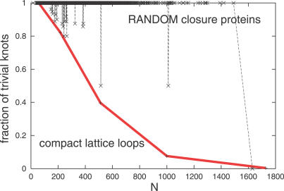
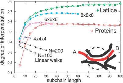
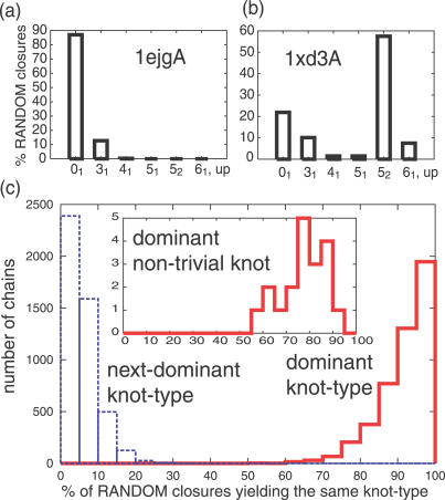
Like shoelaces, the backbones of proteins may get entangled and form knots. However, only a few knots in native proteins have been identified so far. To more quantitatively assess the rarity of knots in proteins, we make an explicit comparison between the knotting probabilities in native proteins and in random compact loops. We identify knots in proteins statistically, applying the mathematics of knot invariants to the loops obtained by complementing the protein backbone with an ensemble of random closures, and assigning a certain knot type to a given protein if and only if this knot dominates the closure statistics (which tells us that the knot is determined by the protein and not by a particular method of closure). We also examine the local fractal or geometrical properties of proteins via computational measurements of the end-to-end distance and the degree of interpenetration of its subchains. Although we did identify some rather complex knots, we show that native conformations of proteins have statistically fewer knots than random compact loops, and that the local geometrical properties, such as the crumpled character of the conformations at a certain range of scales, are consistent with the rarity of knots. From these, we may conclude that the known "protein universe" (set of native conformations) avoids knots. However, the precise reason for this is unknown--for instance, if knots were removed by evolution due to their unfavorable effect on protein folding or function or due to some other unidentified property of protein evolution.

Figure 1. Data for the Mean Square End-to-End Distance of Subchains of Proteins (Squares) and Compact Lattice Loops (Circles) Plotted against the Subchain Length in a log–log Scale

The mean square end-to-end distance of subchains for compact lattice loops of sizes 4 × 4 × 4, 6 × 6 × 6, and 8 × 8 × 8 also are shown to illustrate saturation at different loop sizes. For each chain of length N, subchains of length up to N ^2/3 contribute to the average. The dashed line corresponds to a random walk behavior 〈R ²(ℓ)〉 = ℓ. The mean square end-to-end distance in Ų for proteins has been divided by the factor (3.8)². The data for proteins is similar to that in Figure 2 of [14]. (In that work, the end-to-end distance instead of the square of the end-to-end distance is plotted). The inset at the upper left shows the local scaling exponent 2ν, where 〈R ²(ℓ)〉 ∼ ℓ ^2ν, plotted against subchain length (up to 80 residues) for proteins. 2ν was calculated from two adjacent protein data points at ℓ ₁ and ℓ ₂ via 2ν = log [〈R ²(ℓ ₂)〉/〈R ²(ℓ ₁)〉]/log(ℓ ₂ /ℓ ₁). The horizontal dashed line in the inset represents the exponent 2ν = 1.

Figure 2. Fraction of Protein Chains at a Given Length with a Trivial Knot (0₁) in the RANDOM Method, Plotted against the Length or Number of Residues

Adjacent points are connected by dashed lines. The data for the trivial knotting probability of compact lattice loops (from 4 × 4 × 4 to 12 × 12 × 12) is included, shown connected by thick lines.

Figure 3. Degree of Interpenetration of Subchains

Defined as follows: given a labeled subchain (say chain AB in the inset at the lower right), determine the fraction of the number of units (or residues) of the loop or protein enclosed within a sphere (dashed circle) that does not belong to the subchain. The radius of this enclosing sphere is equal to the gyration radius of the subchain. The degree of interpenetration is then defined as an average of this quantity over all subchains of the given length, taken within a single protein chain and from all other protein chains. As in the results for the mean square end-to-end distance, for each chain of length N, we consider subchains of length up to N^2/3. The degree of interpenetration for proteins, lattices (average from five globular loop sizes from 4 × 4 × 4 to 12 × 12 × 12, and separately for 4 × 4 × 4, 6 × 6 × 6, and 8 × 8 × 8) and linear equilateral random walks of length N = 100 and N = 200 are shown.

Figure 4. Dominance of Knot Types in the RANDOM Knot Closure

(A) Percentage of the 1,000 RANDOM chain closures yielding the various knot types for the protein chain with ID 1ejgA and length N = 46. In this chain, the trivial knot or unknot (0₁) dominates, while the trefoil knot (3₁) is the next-dominant knot type. Both CENTER and DIRECT methods also predict a trivial knot. (B) Percentage of the 1,000 RANDOM chain closures yielding the various knot types for the protein chain with ID 1xd3A and length N = 229. In this chain, the knot 5₂ dominates, while the trivial knot is the next-dominant knot type. The CENTER method also predicts a 5₂ knot, while the DIRECT method detects a trivial knot. (C) Histogram of the percentage of RANDOM chain closures giving the dominant (solid steps) and next-dominant (dashed boxes) knot types within a single chain for all 4,716 protein chains. The inset shows the histogram for the percentage of closures giving the dominant knot type that is not a trivial knot.

Figure 5. Distribution of the Distance of a Protein Terminal from the Center of Mass (R_T)

(R_max is the distance of the residue farthest from the center of mass of the protein chain.) The distribution is divided by (R_T/R_max)² to obtain a density and to take into account that a point chosen at random within a sphere is more likely to be found away from the center of the sphere.

Figure 6. Illustration of the Three Chain Closure Methods

The examples in these figures use the protein chain with PDB ID 1ejgA, rendered using Rasmol (R. Sayle). (A) DIRECT method. T ₁ and T ₂ refer to the terminals of the chain. We connect the terminals by the straight segment T ₁ – T ₂. (B) CENTER method. We enclose the entire chain in a sphere centered at C, the center of mass of the chain. We take straight lines starting at C, passing through the terminals T ₁ and T ₂, and intersecting the surface of the enclosing sphere at the points S ₁ and S ₂. S ₁ and S ₂ are connected to point F, located sufficiently far away outside the sphere, on the plane formed by C, S ₁, and S ₂. The closed loop is formed by the protein chain backbone complemented by the broken line T ₁ − S ₁ − F − S ₂ − T ₂. (C) RANDOM method. The points S ₁ and S ₂ are randomly positioned on the surface of the enclosing sphere whose center coincides with the center of mass of the chain. S ₁ and S ₂ are connected to point F, located sufficiently far away outside the sphere, on the plane formed by the center of mass, S ₁ and S ₂. A closed loop is again formed by the protein chain backbone complemented by the broken line T ₁ − S ₁ − F − S ₂ − T ₂.

References

1. Mansfield ML. Are there knots in proteins? Nat Struct Biol. 1994;1:213–214. - PubMed
1. Mansfield ML. Fit to be tied. Nat Struct Biol. 1997;4:166–167. - PubMed
1. Taylor WR. A deeply knotted protein and how it might fold. Nature. 2000;406:916–919. - PubMed
1. Taylor WR, Lin K. A tangled problem. Nature. 2003;421:25. - PubMed
1. Taylor WR, May ACW, Brown NP, Aszodi A. Protein structure: Geometry, topology and classification. Rep Prog Phys. 2001;64:517–590.
Publication types