The statistical computation underlying contrast gain control

Abstract

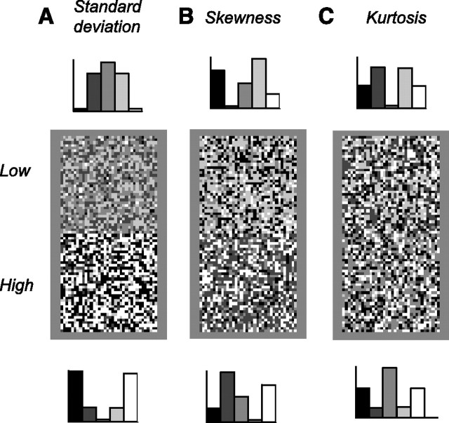
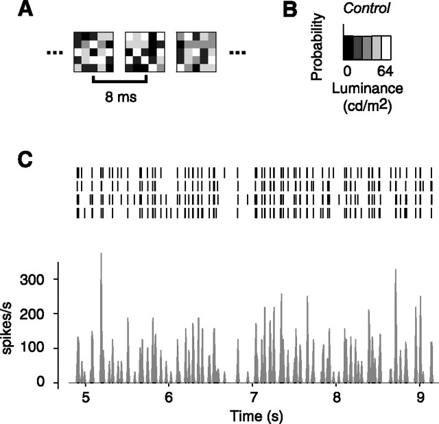
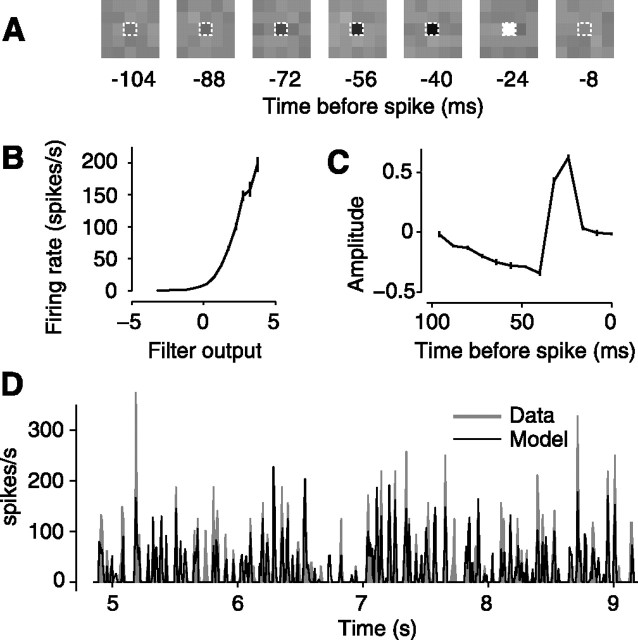
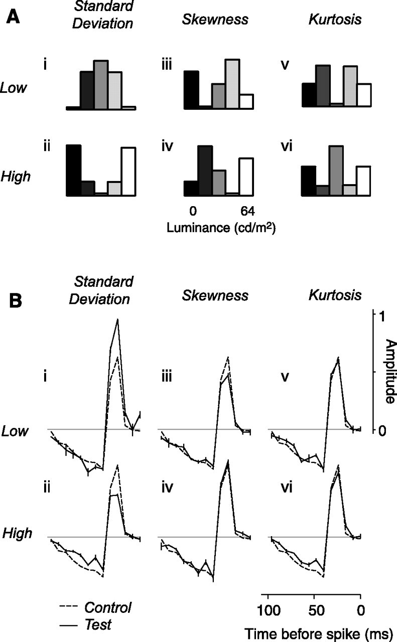
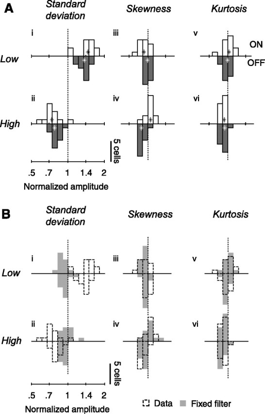
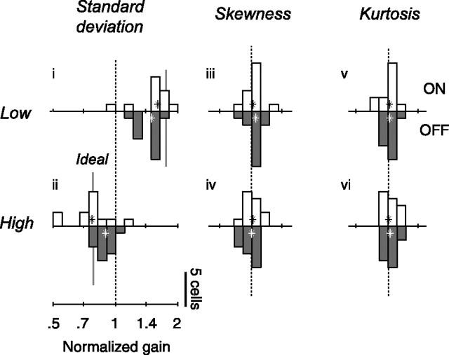
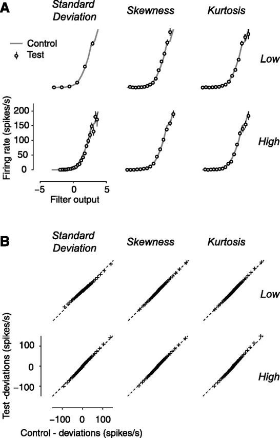
In the early visual system, a contrast gain control mechanism sets the gain of responses based on the locally prevalent contrast. The measure of contrast used by this adaptation mechanism is commonly assumed to be the standard deviation of light intensities relative to the mean (root-mean-square contrast). A number of alternatives, however, are possible. For example, the measure of contrast might depend on the absolute deviations relative to the mean, or on the prevalence of the darkest or lightest intensities. We investigated the statistical computation underlying this measure of contrast in the cat's lateral geniculate nucleus, which relays signals from retina to cortex. Borrowing a method from psychophysics, we recorded responses to white noise stimuli whose distribution of intensities was precisely varied. We varied the standard deviation, skewness, and kurtosis of the distribution of intensities while keeping the mean luminance constant. We found that gain strongly depends on the standard deviation of the distribution. At constant standard deviation, moreover, gain is invariant to changes in skewness or kurtosis. These findings held for both ON and OFF cells, indicating that the measure of contrast is independent of the range of stimulus intensities signaled by the cells. These results confirm the long-held assumption that contrast gain control computes root-mean-square contrast. They also show that contrast gain control senses the full distribution of intensities and leaves unvaried the relative responses of the different cell types. The advantages to visual processing of this remarkably specific computation are not entirely known.

Figure 1.

White noise textures differing in standard deviation, skewness, and kurtosis. Each rectangle contains two squares, one for each value of the statistic being considered. The histograms on the top and bottom indicate the associated distribution of light intensities, i.e., the probability of having a pixel of a certain intensity as a function of intensity. A, Textures differing in standard deviation (root-mean-square contrast) and kurtosis. B, Textures differing only in skewness. C, Textures differing only in kurtosis. The methods to synthesize these textures were introduced by Chubb et al. (1994).

Figure 2.

Measuring LGN responses to the white noise textures. This figure illustrates responses to the control texture, which has uniform distribution. A, Some frames of the texture stimulus. B, Distribution of light intensities. C, Responses of an example LGN neuron (cell 51.3.1) to the texture stimulus. The raster plot indicates spike response in individual trials. The histogram shows firing rate response averaged across trials.

Figure 3.

A simple linear filter followed by a static nonlinearity describes the operation and the responses of the neuron. For the same neuron as in Figure 2, we here illustrate responses to the control texture, which has uniform distribution. A, Estimated linear filter. The dashed contour indicates the location at which the filter has maximal amplitude. B, Estimated static nonlinearity; measured mean firing rate for a given filter output. Error bars (barely visible) indicate ± 1 SE. C, Time course of filter component with maximal amplitude. Error bars (barely visible) indicate ± 1 standard deviation calculated across trials. D, Shaded areas indicates measured firing response. The solid lines indicates model predictions.

Figure 4.

Distribution of light intensities in the test conditions, and results for the example neuron. A, Distribution of light intensities in the six test conditions: low and high standard deviation (i, ii), low and high skewness (iii, iv), and low and high kurtosis (v, vi). B, Results for the example neuron from Figures 2 and 3. The solid curves show the temporal weighting functions measured for each of the test conditions. The dashed curve indicates the time course measured in the control condition (Fig. 3C).

Figure 5.

Changes in response amplitude for the population of neurons (n = 25) and for simulated neurons in which gain is constant. A, Amplitude of responses in the six test conditions, relative to amplitude in the control condition. Open and closed histograms show gain of ON and OFF cells. Stars denote medians across cells. Amplitude is defined as the standard deviation of the temporal weighting function as estimated by spike-triggered averaging. B, Shaded areas show distribution of amplitude changes predicted by a linear–nonlinear Poisson model with fixed temporal weighting function. The dashed histograms are replotted from A.

Figure 6.

Changes in neuronal gain for the population of neurons (n = 25), the same as in Figure 5 except that open and closed histograms show for ON and OFF cells the ratios of observed amplitude changes over those predicted by the linear nonlinear Poisson model.

Figure 7.

Model performance. A, The nonlinearity is approximately constant across stimulus conditions. Results for the example neuron of Figures 2, 3, and 4. Data points indicate the nonlinearities measured in the test conditions. The gray curve indicates the nonlinearity measured in the control condition (Fig. 3B). B, The quality of model predictions is similar across conditions. Results for the population of neurons (n = 25) are shown. Data points indicate quantiles of deviations in test conditions as a function of quantiles observed in the control condition. The dashed lines indicate unity relationship.

References

1. Baccus SA, Meister M (2002). Fast and slow contrast adaptation in retinal circuitry. Neuron 36:909–919. - PubMed
1. Benardete EA, Kaplan E (1999). The dynamics of primate M retinal ganglion cells. Vis Neurosci 16:355–368. - PubMed
1. Benardete EA, Kaplan E, Knight BW (1992). Contrast gain in the primate retina: P cells are not X-like, some M cells are. Vis Neurosci 8:483–486. - PubMed
1. Bonin V, Mante V, Carandini M (2005). The suppressive field of neurons in lateral geniculate nucleus. J Neurosci 25:10844–10856. - PMC - PubMed
1. Brainard DH (1997). The psychophysics toolbox. Spat Vis 10:433–436. - PubMed
Publication types
LinkOut - more resources