Multi-area visuotopic map complexes in macaque striate and extra-striate cortex

Abstract

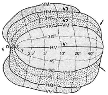
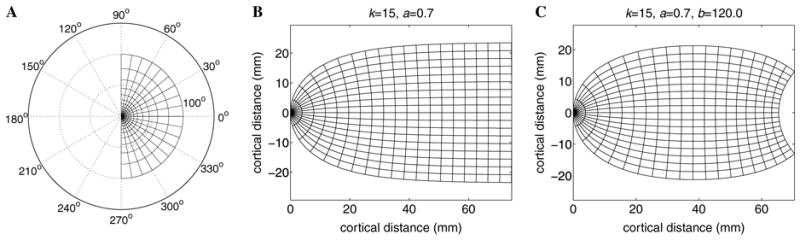
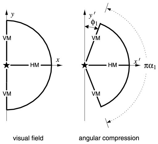
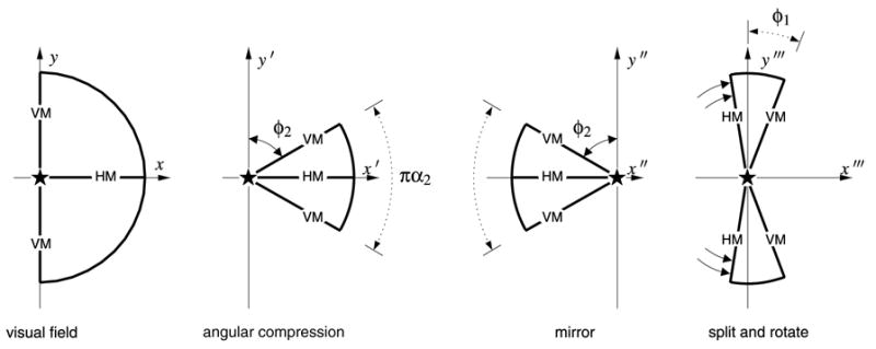
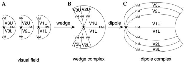
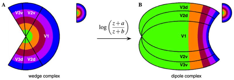
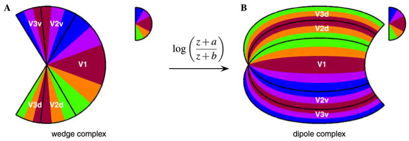
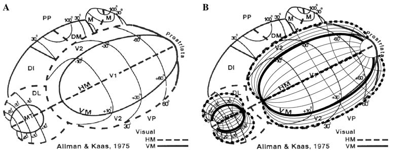
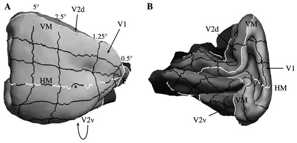
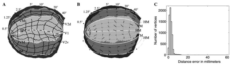
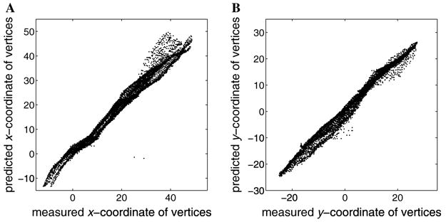
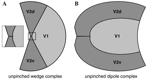
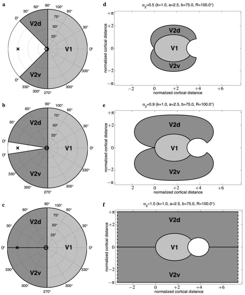
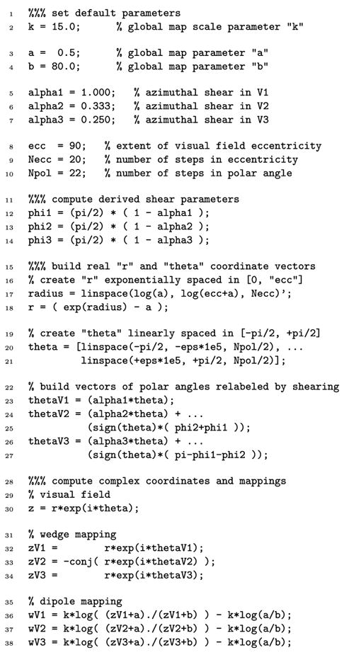
We propose that a simple, closed-form mathematical expression-the Wedge-Dipole mapping-provides a concise approximation to the full-field, two-dimensional topographic structure of macaque V1, V2, and V3. A single map function, which we term a map complex, acts as a simultaneous descriptor of all three areas. Quantitative estimation of the Wedge-Dipole parameters is provided via 2DG data of central-field V1 topography and a publicly available data set of full-field macaque V1 and V2 topography. Good quantitative agreement is obtained between the data and the model presented here. The increasing importance of fMRI-based brain imaging motivates the development of more sophisticated two-dimensional models of cortical visuotopy, in contrast to the one-dimensional approximations that have been in common use. One reason is that topography has traditionally supplied an important aspect of "ground truth," or validation, for brain imaging, suggesting that further development of high-resolution fMRI will be facilitated by this data analysis. In addition, several important insights into the nature of cortical topography follow from this work. The presence of anisotropy in cortical magnification factor is shown to follow mathematically from the shared boundary conditions at the V1-V2 and V2-V3 borders, and therefore may not causally follow from the existence of columnar systems in these areas, as is widely assumed. An application of the Wedge-Dipole model to localizing aspects of visual processing to specific cortical areas-extending previous work in correlating V1 cortical magnification factor to retinal anatomy or visual psychophysics data-is briefly discussed.

Fig. 1

The topography of human visual areas V1, V2, and V3. The “HM” and “VM” mark the representations of the horizontal and vertical meridians, respectively. Iso-eccentricity contours run roughly vertically in this layout, and iso-azimuthal contours run roughly horizontally. Reproduced from Horton and Hoyt (1991a).

Fig. 2

Iso-azimuth and iso-eccentricity contours mapped through the two complex logarithm models of V1 topography. (A) The right visual hemi-field. Visual field coordinates representing eccentricity and azimuth appear as labeled iso-contours, with the foveal representation at the origin. (B) The a-monopole map of the right visual hemi-field. (C) The ab-dipole map of the right visual hemi-field. In each diagram, eccentricity increases from left to right. Note that the iso-azimuth contours are located uniformly in visual field coordinates, whereas the iso-eccentricity contours are exponentially located.

Fig. 3

The wedge mapping for V1 consists of an angular compression of the contralateral visual hemi-field by a factor of α₁ such that the visual hemi-field maps to a wedge-shaped representation of equal radius. The labels “HM” and “VM” mark the horizontal meridian and vertical meridian representations, respectively, and the “★” denotes the location of the foveal representation.

Fig. 4

The wedge mapping for V2 requires extra steps to induce the field reversal and to meet the boundary condition imposed by V1. The angular compression of the contralateral visual hemi-field by the factor of α₂ maps the visual hemi-field into a wedge-shaped representation of equal radius. Then, the wedge is mirrored about the y axis. Finally, the compressed wedge is split along the horizontal meridian representation into half-wedges representing the upper hemi-field and lower hemi-field, which are then each rotated away from the negative x axis until the vertical meridian representation aligns with that of the V1 wedge, shown in Fig. 3. Note that the angle φ₁ represents the angle between the vertical meridian representation and the y axis in the V1 wedge map. The labels “HM” and “VM” mark the horizontal meridian and vertical meridian representations, respectively, and the “★” denotes the location of the foveal representation.

Fig. 5

Schematic of the mapping composition. (A) Three copies of the contralateral visual field (one each for V1, V2, and V3) are mapped into the wedges shown in (B) by the wedge map. The dipole map is then applied to the wedges, resulting in the full Wedge–Dipole map, shown in (C). The “★” denotes the location of the foveal representation. The quadrants of each visual hemi-field are labeled as “V1U,” “V2U,” and “V3U” for the upper field, and “V1L,” “V2L,” and “V3L” for the lower field. The horizontal meridian and vertical meridian are labeled as “HM” and “VM,” respectively.

Fig. 6

Schematic visual field eccentricity mapping into the wedge complex and the dipole complex. (A) The eccentricity of the visual field for the combined wedge complex for V1, V2, and V3 demonstrates that the azimuthal compression induced by the wedge mapping changes the azimuth but does not affect eccentricity. The representation of eccentricity is also shown to be continuous across the region boundaries. (B) The visual field representation in cortical space, after applying the dipole mapping to the wedge complex. The eccentricity of the internal topographic representation demonstrates the magnification of the foveal representation as well as the compression of the periphery in all three regions shown. Additionally, the iso-eccentricity bands are shown to intersect each region boundary orthogonally and to be continuous across the boundaries. The half-disc inset in the upper right of each panel provides the eccentricity on the visual hemi-field in pseudocolor.

Fig. 7

Schematic of the visual field azimuth mapping into the wedge complex and the dipole complex. (A) The azimuth of the visual field for the combined wedge complex consists of the wedge mappings of V1, V2, and V3, demonstrating the azimuthal compression of the visual field as well as the field reversal across wedge boundaries. (B) The outcome of applying the dipole mapping to the wedge complex shows the field reversal property in cortical coordinates: across any given border between two cortical regions the direction of increasing azimuth reverses. The V1/V2 border represents the vertical meridian of the visual field, whereas the V2/V3 border represents the horizontal meridian, resulting in the the ventral half of the cortical space representing the upper quadrant of the visual field and the dorsal half representing the lower quadrant. The labels “V2v” and “V3v” indicate the ventral halves of V2 and V3, and “V2d” and “V3d” indicate the dorsal halves. The half-disc inset in the upper right of each panel provides the azimuth on the visual hemi-field in pseudocolor.

Fig. 8

The topography of human visual areas V1, V2, and V3 from Horton and Hoyt (1991a) (as shown in Fig. 1) with the iso-eccentricity and iso-azimuth contours predicted by the Wedge–Dipole model superimposed on the three areas. The model parameters used here were a = 0.9°, b = 180°, α₁ = 0.95, α₂ = 0.5, and α₃ = 0.2. The value of a here is somewhat higher than we have found for quantitative analysis of macaque and human, possibly due to the semi-quantitative nature of this data set. The representation of the horizontal meridian in the Wedge–Dipole model is shown with thick dashed lines, and the representation of the vertical meridian is shown with thick solid lines.

Fig. 9

The topography of owl monkey visual cortex is shown in (A) from the data of Allman and Kaas (1975) (reproduced from Kaas, 1997, chap. 3). Two Wedge–Dipole maps are shown superimposed on this data set in (B), one for the V1–V2 complex (model parameters a = 0.8°, b = 85°, α₁ = 1.05, and α₂ = 0.33), and one for the MT–DL complex (model parameters a = 10°, b = 70°, α₁ = 1, and α₂ = 0.5). The MT–DL model has been scaled by a factor of 0.65 relative to the V1–V2 model. “HM” and “VM” mark the cortical representation of the horizontal meridian and vertical meridian, respectively, in the data. The representation of the horizontal meridian in the Wedge–Dipole model is shown with thick dashed lines, and the representation of the vertical meridian is shown with thick solid lines.

Fig. 10

(A) Visuotopy data obtained from tangential section through layer IV of physically flattened macaque V1 of right hemisphere. (B) The visuotopic mapping stimulus consisted of a ring and ray pattern of black-and-white checks and subtended approximately 20° of the visual field. (C) Nearisometrically flattened computer reconstruction of macaque V1 visuotopy data from the left hemisphere of the same macaque. The local coordinate directions for the opercular cortex are given in the legend. Abbreviations: cas, calcarine sulcus; lus, lunate sulcus; ios, inferior occipital sulcus; and lcs, lateral calcarine sulcus.

Fig. 11

(A) The numbered red circles mark features of the visual stimulus within the right hemi-field identified in the 2DG labeling of V1 that were used for the model fit. (B) Computer reconstruction of V1 from the left hemisphere. The 2DG-labeled activity pattern from layer IV was texture mapped onto numerically flattened V1 surface mesh. The numbered blue squares correspond to the locations of the visual stimulus features shown in (A).

Fig. 12

Monopole model fits to computer-reconstructed macaque visuotopy. (A) Comparison between optimal model fit and data. The model parameters were obtained by minimizing the RMS error between the model prediction and the data. The blue squares mark the data points, the red circles mark the model prediction for each data point, and the red line segments connect corresponding measurement-prediction pairs. The black dashed lines represent the predicted locations of the rings and rays of the visual stimulus, which match the imprinted representation of the stimulus in the data well. (B) Plot of the measured versus predicted coordinate values for each data point. The correlation coefficient for the position along the anterior–posterior axis and the position along the dorsal–ventral axis was 0.98 and 0.99, respectively, indicating that the model was able to account for the variance in the data and thus provided a good fit.

Fig. 13

(A) A lateral view of V1 (light gray) and V2 (medium gray) of macaque visual cortex. (B) A medial view of V1 and V2, exposing the calcarine sulcus. Several iso-eccentricity and iso-azimuth contours are shown (as solid lines) on the cortical surface. “HM” (dashed white line) and “VM” (solid white line) mark the cortical representation of the horizontal meridian and vertical meridian, respectively, and “F” marks the representation of the fovea. “V1” marks striate cortex, and “V2d” and “V2v” mark dorsal and ventral V2, respectively. The topography of V1 and V2 is easier to visualize on a flattened representation of these areas, as shown in Fig. 14A.

Fig. 14

(A) Near-isometric flattening of macaque V1 (light gray) and V2 (medium gray), with several iso-eccentricity and iso-azimuth contours shown as black lines. “HM” and “VM” mark the cortical representation of the horizontal meridian and vertical meridian, respectively, and “F” marks the representation of the fovea. “V1” marks striate cortex, and “V2d” and “V2v” mark dorsal and ventral V2, respectively. (B) The corresponding iso-eccentricity and iso-azimuth contours are shown (as dotted lines) for a fit of the Wedge–Dipole map to the data in (A). The model parameters were obtained by minimizing the RMS value of the error per vertex. The short black line segments indicate displacements from the intersections of the iso-eccentricity lines with the iso-azimuth lines in the model to the corresponding locations in the data in (A). The black squares correspond to locations where the lines in (A) do not intersect due to missing data. (C) A histogram of modeling errors (i.e., distances between the data and the model predictions).

Fig. 15

The results of minimizing the RMS error of the Wedge–Dipole model fit to V1 and V2 topography in the F99UA1 data set. The cortical coordinates of the data points plotted against model predictions for (A) the x coordinate and (B) the y coordinate.

Fig. 16

(A) “Unpinching” the wedge complex consists of moving the complex to the right of the origin then bending the complex around the origin. The inset shows a close-up of the unpinched wedge complex at the foveal representation. (B) The result of mapping the unpinched wedge complex through the dipole mapping is a dipole complex in which the the foveal representation in V2 assumes more cortical area (cf. Fig. 1).

Fig. 17

Representation of monocular component of the visual hemi-field in V1 under the dipole mapping. (A) A qualitative model of the right visual hemi-field, with the monocular and binocular fields demarcated (cf. Polyak, 1941). (B) The representation of both the binocular and monocular visual hemi-field components in primary visual cortex under the Wedge–Dipole mapping. The outline of the monocular field representation, appearing in the peripheral area of V1, fills in the concave gap in the dipole mapping and resembles the anatomical shape of the monocular crescent.

Fig. 18

Wedge–Dipole model with alternate azimuthal shear distribution. This extension includes a non-uniformity in the azimuthal shear term that induces greater azimuthal shear along the area boundaries. V1 is shown in light gray, V2 in medium gray, and V3 in dark gray. The solid lines internal to the areas represent the iso-azimuth contours of the visuotopic mapping, and the dotted lines represent the iso-eccentricity contours. The shear non-uniformity manifests as a tighter spacing of the iso-azimuth contours near the area boundaries (cf. Fig. 2C). The particular non-uniformity shown here corresponds to a sigmoidal compression near to the boundaries and expansion in the interior.

Fig. 19

Demonstration of the effect of logarithmic singularities on V2 surface area under Wedge–Dipole mapping as a function of the azimuthal shear parameter, α₂. Each row depicts a pair of wedge and dipole complexes corresponding to a given value of α₂. (A–C) The wedge complex representation of the right hemi-field of V1 and V2. Visual field coordinates representing eccentricity and azimuth appear as labeled iso-contours, with the foveal representation at the origin. The location of the logarithmic singularities corresponding to the a and b dipole parameters is denoted with the symbols “○” and “×,” respectively. (D–F) The cortical representation of the two visual areas under the wedge and dipole mappings. In each dipole mapping depicted above, the mapping parameters were k = 1 mm/°, a = 2.5°, and b = 75°, with a maximum eccentricity of 100 ° and zero azimuthal shear in V1, α₁ = 0 (see Mathematical Appendix for explanation of mapping parameters). (D) A moderate amount of azimuthal shear in V2 (α₂ = 0.5) causes the area of V2 under the dipole to be comparable to that of V1, as is observed in the existing macaque data. (E) Applying less azimuthal shear (α₂ = 0.9) results in the borders of the wedge representation closing in on the singularities, leading to a dramatic expansion of area in V2. (F) Finally, when the shear is reduced enough to allow the wedge representation of V2 to approach the singularities (α₂ = 1), the area of the V2 cortical representation becomes infinite (see Section 4.3.1). The dashed lines represent the V2 boundary segment at infinity. This is the case in which both V1 and V2 are simultaneously conformal.

Fig. 20

Example MATLAB code for Wedge–Dipole mapping.

References

1. Adams DL, Horton JC. “What you see …”, review of Visual Disturbances following Gunshot Wounds of the Cortical Visual Areaby Tatsuji Inouye (M. Glickstein, & M. Fahle, Trans) Nature. 2001;412(6846):482–483.
1. Adams DL, Horton JC. Shadows cast by retinal blood vessels mapped in primary visual cortex. Science. 2002;298(5593):572–576. - PMC - PubMed
1. Adams DL, Horton JC. Capricious expression of cortical columns in the primate brain. Nature Neuroscience. 2003a;6(2):113–114. - PubMed
1. Adams DL, Horton JC. A precise retinotopic map of primate striate cortex generated from the representation of angioscotomas. Journal of Neuroscience. 2003b;23(9):3771–3789. - PMC - PubMed
1. Ahlfors LV. Complex analysis. 2. New York: McGraw-Hill; 1966a.
Publication types