Complex parameter landscape for a complex neuron model

Abstract

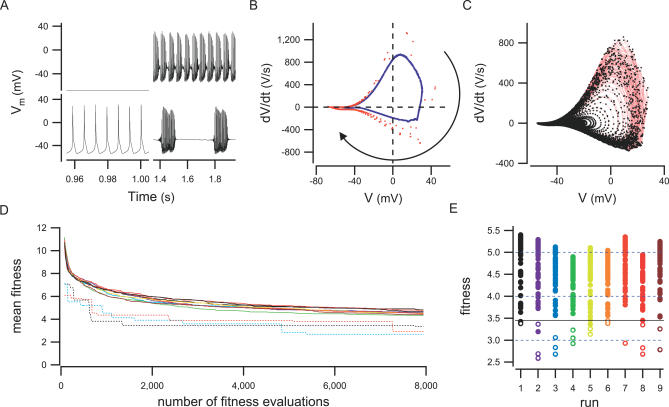
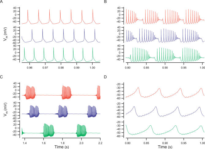
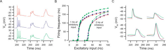
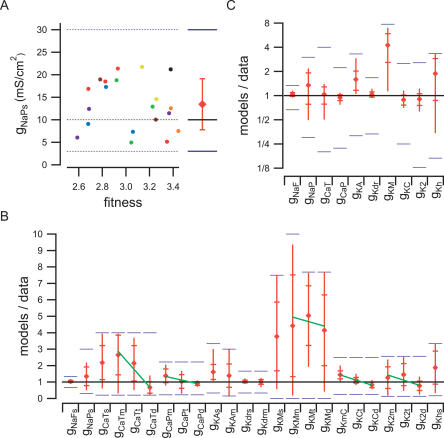
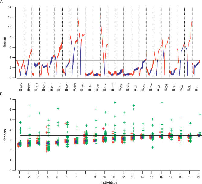
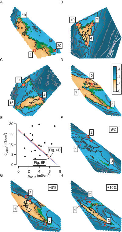
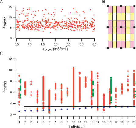
The electrical activity of a neuron is strongly dependent on the ionic channels present in its membrane. Modifying the maximal conductances from these channels can have a dramatic impact on neuron behavior. But the effect of such modifications can also be cancelled out by compensatory mechanisms among different channels. We used an evolution strategy with a fitness function based on phase-plane analysis to obtain 20 very different computational models of the cerebellar Purkinje cell. All these models produced very similar outputs to current injections, including tiny details of the complex firing pattern. These models were not completely isolated in the parameter space, but neither did they belong to a large continuum of good models that would exist if weak compensations between channels were sufficient. The parameter landscape of good models can best be described as a set of loosely connected hyperplanes. Our method is efficient in finding good models in this complex landscape. Unraveling the landscape is an important step towards the understanding of functional homeostasis of neurons.

Figure 1. The Search Method

(A) Example of the four firing modes of the PC: silent (top left), tonic (bottom left), small bursts (top right), and long bursts (bottom right) obtained with respectively 0, 0.5, 2, and 3 nA of current injected in the soma. (B) The (V,dV/dt) matrix obtained for data when a current of 0.5 nA is injected in the soma. The red points correspond to the first 0.1 s after current injection (transitory period), while the blue ones represent 1.1 s of data recorded 0.9 s after the beginning of current injection (stable period). The black arrow shows the direction followed by successive points in time during a spike. (C) The (V,dV/dt) matrix obtained for data when a current of 3 nA is injected in the soma. The black points represent 2.1 s of data recorded 0.9 s after the beginning of current injection. The red lines link successive points. (D) Time evolution of the mean fitness of the population (full lines). The nine runs, shown as different colors, have very similar evolution, and were stopped after 415 generations. The time evolution of the fitness of the best individual of runs 1, 3, and 7 is shown as dashed lines. (E) Fitness of all individuals of each population when the runs were stopped. Open points represent individuals selected for the rest of the analysis. The full line corresponds to the fitness upper limit for selecting individuals.

Figure 2. Comparison of the Models with the Data for Current Clamp

(A–C) The membrane potential of the soma is shown for the data (red traces), best (blue), and worst (green) model of our selection for different somatic current amplitudes: 0.5 (A), 2 (B), and 3 nA (C). (D) Same as (B) for dendritic membrane potential.

Figure 3. Comparison of the Models with the Data for Synaptic Responses

Data (red lines), best (blue lines), and worst (green lines) model of our selection are compared for different synaptic responses. (A) Complex spike in the soma (left), main dendrite (middle), and smooth dendrite (right) after activation of the climbing fiber at time 0.2 s. (B) Simple spike frequency response to different levels of excitation and inhibition. (C) EPSPs generated by a synchronous parallel fiber input plus an asynchronous background excitation and inhibition. EPSPs are generated in four different branchlets and recorded at the soma, which is passive. The traces show the average of 40 EPSPs obtained with different random number generator seeds.

Figure 4. Conductance Spread

(A) The fitness of each individual is plotted against its g_NaPs value. Points of the same color belong to the same population (see Figure 1E). Blue lines give the range in which channel densities were allowed to vary while the black line gives the value of the data. On the right, the red marker shows the mean ± sdv of the 20 values. (B) For each conductance, the mean value of the 20 selected individuals is shown, normalized to the data. The full red bars delimit the whole range covered by the 20 models while the horizontal red lines give sdv. Blue bars show the range of variation allowed during the search. Green lines are linear fit, supposing regular spacing on the abscissa. (C) Same as (B) for total conductances, obtained by summing conductance densities of the same type, weighted by the surface area of the membrane regions where they apply.

Figure 5. Points of the Parameter Space around the Data and the Selected Individuals

(A) Fitness of 24 × 500 points for which all the parameters are equal to that of the data but one, labeled on the abscissa, and varied randomly in the full allowed range (see Table 1). The mean ± sdv range covered by the 20 selected individuals is shown in blue for each conductance density. The exact data value is never randomly selected so none of the distributions reached the perfect fitness value of 0. (B) For each of the 20 selected individuals (blue dots), the fitness of the 48 individuals obtained by changing its parameters by ±1% (red) or ±5% (green). Only one parameter is changed at a time.

Figure 6. Two-Dimensional Views of Some Hyperplanes of the Parameter Space

(A–D) Some typical projections onto the (g_NaPs, g_NaFs) plane of hyperplanes defined by triplets of individuals. The fitness values of all points belonging to these hyperplanes are color scaled. The three original individuals of each hyperplane are labeled and highlighted by a red square. Grey lines delimitate iso-fitnesses. (E) The hyperplane of (D) is shown in red in projection onto the (g_CaTs, g_CaTd) plane. The 20 best individuals are represented by points. A blue hyperplane is drawn parallel to the red one. It is defined by adding to the red hyperplane points 10% of the sdv of all solutions in every dimension. Note that individuals that are in between these hyperplanes in this projection can be very far away in other dimensions. (F–H) Parallel hyperplanes of (D), with the same projection. These hyperplanes are obtained by adding respectively −5%, +5%, and +10% of sdv to the points belonging to the hyperplane shown in (D). The red cross mark the region of best fitness in the original hyperplane (D).

Figure 7. Comparison with other Methods

(A) Fitness of hundreds of individuals obtained during the searching algorithm evolution, as a function of their g_CaTs value and centered around the data value (equal to 5). (B) Parameter space simplified to a grid of three black points in two dimensions. All individual falling in a pink region will have just one close neighbor, all the points in yellow area will have two close neighbors, and all the points in a white area will have four close neighbors. (C) Depending upon individuals (blue circles), between eight and 4,096 close neighbors are found on a six-points-per-dimension grid. The fitnesses of all these neighbors are shown as red crosses. For some individuals which have neighbors with fitness values above 3.45 but below 4 a grid of ten points per dimension was also tested (green crosses).

References

1. MacLean JN, Zhang Y, Johnson BR, Harris-Warrick RM. Activity-independent homeostasis in rhythmically active neurons. Neuron. 2003;37:109–120. - PubMed
1. Swensen AM, Bean BP. Robustness of burst firing in dissociated Purkinje neurons with acute or long-term reductions in sodium conductance. J Neurosci. 2005;25:3509–3520. - PMC - PubMed
1. Schulz DJ, Goaillard JM, Marder E. Variable channel expression in identified single and electrically coupled neurons in different animals. Nat Neurosci. 2006;9:356–362. - PubMed
1. Prinz AA, Bucher D, Marder E. Similar network activity from disparate circuit parameters. Nat Neurosci. 2004;7:1345–1352. - PubMed
1. Goldman MS, Golowasch J, Marder E, Abbott LF. Global structure, robustness, and modulation of neuronal models. J. Neurosci. 2001;21:5229–5238. - PMC - PubMed
Publication types