Stochastic models of receptor oligomerization by bivalent ligand

Abstract

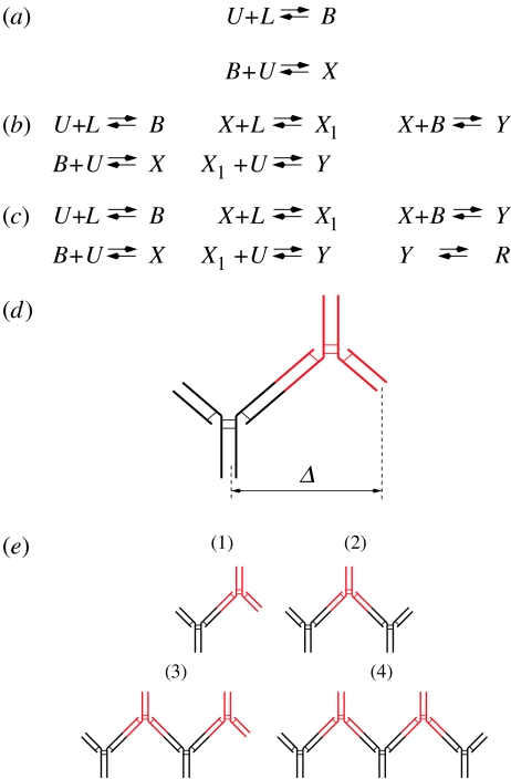
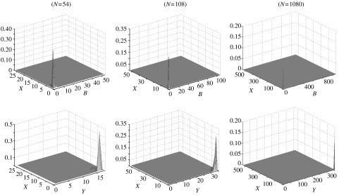
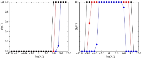
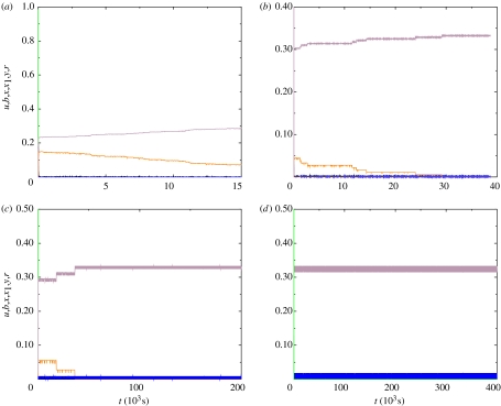
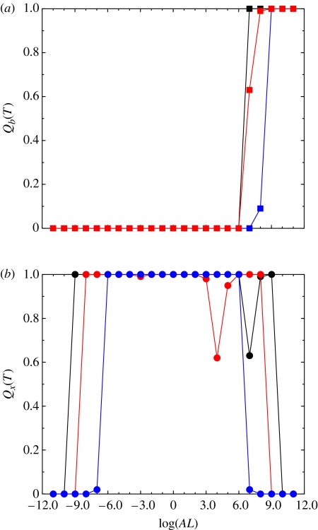
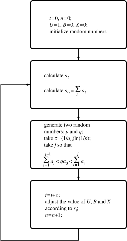
In this paper, we develop stochastic models of receptor binding by a bivalent ligand. A detailed kinetic study allows us to analyse the role of cross-linking in cell activation by receptor oligomerization. We show how oligomer formation could act to buffer intracellular signalling against stochastic fluctuations. In addition, we put forward the hypothesis that formation of long linear oligomers increases the range of ligand concentration to which the cell is responsive, whereas formation of closed oligomers increases ligand concentration specificity. Thus, different physiological functions requiring different degrees of specificity to ligand concentration would favour formation of oligomers with different lengths and geometries. Furthermore, provided that ligand concentration specificity is taken as a design principle, our model enables us to estimate parameters, such as the minimum proportion of receptors, that must engage in oligomer formation in order to trigger a cellular response.

Figure 1

Schematic of the cross-linking model with (a) dimer formation, (b) trimer formation and (c) ring formation. The physical meaning of the parameter Δ is illustrated in (d). B, X, $X_1$ and Y are the number of oligomers of type (1), (2), (3) and (4), as shown in panel (e), respectively. In panels (d) and (e), red colour indicates diffusible ligand, whereas black colour denotes membrane-bound receptor.

Figure 2

Simulation results from a single realization for (a) N=10 000, (b) N=1000, (c) N=100, (d) N=50. Black lines correspond to x, red lines to b, and green lines to u. $L={10}^{-7}$ mol l⁻¹. See appendix A for details of the simulation procedure.

Figure 3

Probability density corresponding to Model 1. (a) N=1000, average over 300 realizations. (b) N=100, average over 700 realizations. (c) N=50, average over 700 realizations. $L={10}^{-7}$ mol l⁻¹. See appendix A for details of the simulation procedure.

Figure 4

Simulation results for Model 1 showing (a) $Q_b(T)$ and (b) $Q_x(T)$ for $T=10k_{\text{off}}^{-1}$ as a function of the dimensionless quantity AL, where A is the affinity and L the ligand concentration. Blue lines correspond to N=108 and $\Theta /N=0.45$, red lines to N=1080 and $\Theta /N=0.045$ and black lines to N=10 800 and $\Theta /N=0.0045$. In each case, we have averaged over 100 realizations.

Figure 5

Simulation results for Model 1 showing $Q_x(T)$ for $T=10k_{\text{off}}^{-1}$ as a function of the dimensionless quantity AL, where A is the affinity and L the ligand concentration. Black lines correspond to N=10 800, red lines to N=1080 and blue lines to N=108. $\Theta /N=0.45$. In each case, we have averaged over 100 realizations.

Figure 6

Simulation results from a single realization corresponding to Model 2. We have taken (a) N=1080, (b) N=540, (c) N=108, (d) N=54. Black lines correspond to x, orange lines to $x_1$, red lines to b, green lines to u and blue lines to y. $L={10}^{-7}$ mol l⁻¹. See appendix A for details of the simulation procedure.

Figure 7

Probability densities for Model 2 for N=54, 108 and 1080. In all of the different cases, we have averaged over realizations. L=10⁻⁷ mol l⁻¹. See appendix A for details of the simulation procedure.

Figure 8

Simulation results for Model 2 showing (a) $Q_b(T)$ and (b) $Q_x(T)$ for $T=10k_{\text{off}}^{-1}$ as a function of the dimensionless quantity AL, where A is the affinity and L the ligand concentration. Black lines correspond to N=10 800 and $\Theta /N=0.0045$, red lines to N=1080 and $\Theta /N=0.045$ and blue lines to N=108 and $\Theta /N=0.45$. In each case, we have averaged over 100 realizations.

Figure 9

Simulation results for Model 2 showing Q_x(T) for $T=10k_{\text{off}}^{-1}$ as a function of the dimensionless quantity AL, where A is the affinity and L the ligand concentration. These results correspond to varying the threshold value of BCRs engaged in cross-linking necessary for building-up a signal. Black corresponds to N=10 800, red to N=1080 and blue to N=108. $\Theta /N=0.45$. In each case, we have averaged over 100 realizations.

Figure 10

Simulation results from a single realization corresponding to Model 3. We have taken (a) N=1080, (b) N=540, (c) N=108, (d) N=54. Black lines correspond to x, red lines to b, green lines to u, blue lines to y and brown lines to r. $L={10}^{-7}$ mol l⁻¹. See appendix A for details of the simulation procedure.

Figure 11

Simulation results from a single realization corresponding to Model 3. We have taken N=1080. Panel (a) corresponds to $L={10}^{-13}$ mol l⁻¹, panel (b) to $L={10}^{-7}$ mol l⁻¹ and panel (c) to $L={10}^{-1}$ mol l⁻¹. Black lines correspond to x, red lines to b, green lines to u, blue lines to y and brown lines to r. $L={10}^{-7}$ mol l⁻¹. See appendix A for details of the simulation procedure.

Figure 12

Simulation results for Model 1 showing (a) $Q_b(T)$ and (b) $Q_x(T)$ for $T=10k_{\text{off}}^{-1}$ as a function of the dimensionless quantity AL, where A is the affinity and L the ligand concentration. Black lines correspond to N=10 800 and $\Theta /N=0.0045$, red lines to N=1080 and $\Theta /N=0.045$ and blue lines to N=108 and $\Theta /N=0.45$. In each case, we have averaged over 100 realizations.

Figure 13

Simulation results for Model 3 showing $Q_x(T)$ for $T=10k_{\text{off}}^{-1}$ as a function of the dimensionless quantity AL, where A is the affinity and L the ligand concentration. These results correspond to varying the threshold value of BCRs engaged in cross-linking necessary for building-up a signal. Black corresponds to N=10 800, red to N=1080 and blue to N=108. $\Theta /N=0.45$. In each case, we have averaged over 100 realizations.

Figure 14

Simulation results showing $Q_x(T)$ for $T=10k_{\text{off}}^{-1}$ as a function of the dimensionless quantity AL, where A is the affinity and L the ligand concentration. These results correspond to varying the threshold value of BCRs engaged in cross-linking necessary for building-up a signal. Blue to $\Theta /N=0.22$ and maroon to $\Theta /N=0.45$ In each case, we have averaged over 100 realizations.

Figure 15

Sensitivity analysis for $A_x$. Simulation results are shown for $Q_x(T)$ the model with trimer formation showing with $T=10k_{\text{off}}^{-1}$ as a function of the quantity $A_x$. $\Theta /N=0.22$ and $AL={10}^3$ (green line), AL=1 (blackline), $AL={10}^{-4}$ (blue line) and $AL={10}^{-5}$ (red line). Circles correspond to results for Model 2 (a), squares to Model 3 (b). We have averaged over 100 realizations.

Figure 16

Flow chart for the ESSA proposed by Gillespie (1977). See text for details.

References

1. Alberts B, Johnson A, Lewis J, Raff M, Roberts K, Walter P. Garland; New York: 2002. Molecular biology of the cell.
1. Banu Y, Watanabe T. Augmentation of antigen receptor-mediated responses by histamine H1 receptor signalling. J. Exp. Med. 1999;189:673–682. doi:10.1084/jem.189.4.673 - DOI - PMC - PubMed
1. Burrage K, Tian T, Burrage P. A multi-scaled approach for simulating chemical reaction systems. Prog. Biophys. Mol. Biol. 2004;85:217–234. doi:10.1016/j.pbiomolbio.2004.01.014 - DOI - PubMed
1. Durrett R, Levin S. The importance of being discrete (and spatial) Theor. Popul. Biol. 1994;46:363–394. doi:10.1006/tpbi.1994.1032 - DOI
1. Gardiner C.W. Springer; Berlin: 1983. Handbook of stochastic methods.
Publication types
LinkOut - more resources