Optical trapping

Abstract

Since their invention just over 20 years ago, optical traps have emerged as a powerful tool with broad-reaching applications in biology and physics. Capabilities have evolved from simple manipulation to the application of calibrated forces on-and the measurement of nanometer-level displacements of-optically trapped objects. We review progress in the development of optical trapping apparatus, including instrument design considerations, position detection schemes and calibration techniques, with an emphasis on recent advances. We conclude with a brief summary of innovative optical trapping configurations and applications.

FIG. 1

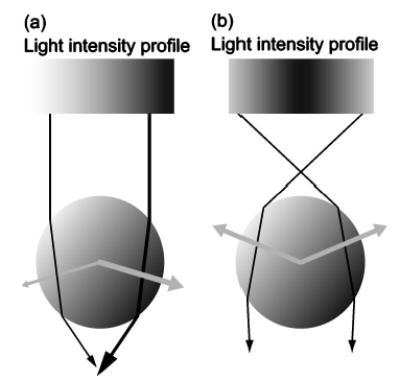
Ray optics description of the gradient force. (A) A transparent bead is illuminated by a parallel beam of light with an intensity gradient increasing from left to right. Two representative rays of light of different intensities (represented by black lines of different thickness) from the beam are shown. The refraction of the rays by the bead changes the momentum of the photons, equal to the change in the direction of the input and output rays. Conservation of momentum dictates that the momentum of the bead changes by an equal but opposite amount, which results in the forces depicted by gray arrows. The net force on the bead is to the right, in the direction of the intensity gradient, and slightly down. (B) To form a stable trap, the light must be focused, producing a three-dimensional intensity gradient. In this case, the bead is illuminated by a focused beam of light with a radial intensity gradient. Two representative rays are again refracted by the bead but the change in momentum in this instance leads to a net force towards the focus. Gray arrows represent the forces. The lateral forces balance each other out and the axial force is balanced by the scattering force (not shown), which decreases away from the focus. If the bead moves in the focused beam, the imbalance of optical forces will draw it back to the equilibrium position.

FIG. 2

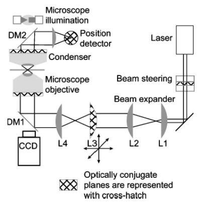
Layout of a generic optical trap. The laser output beam usually requires expansion to overfill the back aperture of the objective. For a Gaussian beam, the beam waist is chosen to roughly match the objective back aperture. A simple Keplerian telescope is sufficient to expand the beam (lenses L1 and L2). A second telescope, typically in a 1:1 configuration, is used for manually steering the position of the optical trap in the specimen plane. If the telescope is built such that the second lens, L4, images the first lens, L3, onto the back aperture of the objective, then movement of L3 moves the optical trap in the specimen plane with minimal perturbation of the beam. Because lens L3 is optically conjugate (conjugate planes are indicated by a cross-hatched fill) to the back aperture of the objective, motion of L3 rotates the beam at the aperture, which results in translation in the specimen plane with minimal beam clipping. If lens L3 is not conjugate to the back aperture, then translating it leads to a combination of rotation and translation at the aperture, thereby clipping the beam. Additionally, changing the spacing between L3 and L4 changes the divergence of the light that enters the objective, and the axial location of the laser focus. Thus, L3 provides manual three-dimensional control over the trap position. The laser light is coupled into the objective by means of a dichroic mirror (DM1), which reflects the laser wavelength, while transmitting the illumination wavelength. The laser beam is brought to a focus by the objective, forming the optical trap. For back focal plane position detection, the position detector is placed in a conjugate plane of the condenser back aperture (condenser iris plane). Forward scattered light is collected by the condenser and coupled onto the position detector by a second dichroic mirror (DM2). Trapped objects are imaged with the objective onto a camera. Dynamic control over the trap position is achieved by placing beam-steering optics in a conjugate plane to the objective back aperture, analogous to the placement of the trap steering lens. For the case of beam-steering optics, the point about which the beam is rotated should be imaged onto the back aperture of the objective.

FIG. 3

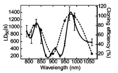
The wavelength dependence of photodamage in E. coli compared to Chinese hamster ovary (CHO) cells. (Solid circles and solid line, left axis, half lethal dose time for E. coli cells (LD₅₀); open circles and dashed line, right axis, cloning efficiency in CHO cells determined by Liang et al. (Ref. 96) (used with permission). Lines represent cubic spline fits to the data). The cloning efficiency in CHO cells was determined after 5 min of trapping at 88 mW in the specimen plane (error bars unavailable), selected to closely match to our experimental conditions (100 mW in the specimen plane, errors shown as ± standard error in the mean). Optical damage is minimized at 830 and 970 nm for both E. coli and CHO cells, whereas it is most severe in the region between 870 and 930 nm (reprinted from Ref. 95).

FIG. 4

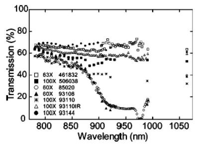
Microscope objective transmission curves. Transmission measurements were made by means of the dual-objective method. Part numbers are cross-referenced in Table I. The uncertainty associated with a measurement at any wavelength is ~5% (reprinted from Ref. 95).

FIG. 5

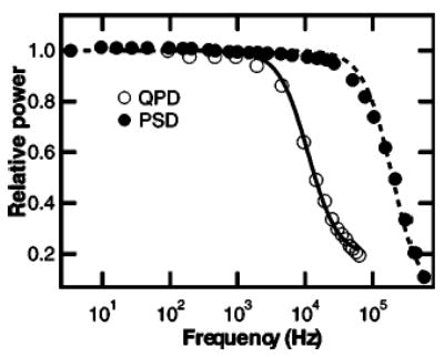
Comparison of position detector frequency response at 1064 nm. Normalized frequency dependent response for a silicon quadrant photodiode (QPD) (QP50–6SD, Pacific Silicon Sensor) (open circles), and a position sensitive detector (PSD), (DL100–7PCBA, Pacific Silicon Sensor) (solid circles). 1064 nm laser light was modulated with an acousto-optic modulator and the detector output was recorded with a digital sampling scope. The response of the QPD was fit with the function: γ²+(1−γ²)[1+(f/f₀)²]⁻¹, which describes the effects of diffusion of electron-hole pairs created outside the depletion layer (Ref. 134), where γ is the fraction of light absorbed in the diode depletion layer and f₀ is the characteristic frequency associated with light absorbed beyond the depletion layer. The fit returned an f₀ value of 11.1 kHz and a γ parameter of 0.44, which give an effective f_3dB of 4.1 kHz, similar to values found in Ref. for silicon detectors. The QPD response was not well fit by a single pole filter response curve. The PSD response, in contrast, was fit by a single pole filter function, returning a rolloff frequency of 196 kHz. Extended frequency response at 1064 nm has also been reported for InGaAs and fully depleted silicon photodiodes (Ref. 61).

FIG. 6

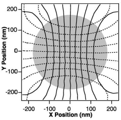
Lateral two-dimensional detector calibration (adapted from Ref. 59). Contour plot of the x (solid lines) and y (dashed lines) detector response as a function of position for a 0.6 μm polystyrene bead raster scanned through the detector laser focus by deflecting the trapping laser with acousto-optic deflectors. The bead is moved in 20 nm steps with a dwell time of 50 ms per point while the position signals are recorded at 50 kHz and averaged over the dwell time at each point. The x contour lines are spaced at 2 V intervals, from 8 V (leftmost contour) to −8 V (rightmost contour). The y contour lines are spaced at 2 V intervals, from 8 V (bottom contour) to −8 V (top contour). The detector response surfaces in both the x and y dimensions are fit to fifth order two-dimensional polynomials over the shaded region, with less than 2 nm residual root mean square (rms) error. Measurements are confined to the shaded region, where the detector response is single valued.

FIG. 7

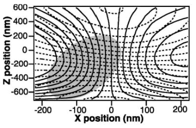
Axial two-dimensional detector calibration. Contour plot of the lateral (solid lines) and axial (dashed lines) detector response as a function of x (lateral displacement) and z (axial displacement) of a stuck 0.5 μm polystyrene bead moving through the laser focus. A stuck bead was raster scanned in 20 nm steps in x and z. The detector signals were recorded at 4 kHz and averaged over 100 ms at each point. The lateral contour lines are spaced at 1 V intervals, from −9 V (leftmost contour) to 7 V (rightmost contour). The axial contour lines are spaced at 0.02 intervals (normalized units). Measurements are confined to the region of the calibration shaded in gray, over which the surfaces of x and z positions as a function of lateral and axial detector signals were fit to seventh order two-dimensional polynomial functions with less than 5 nm residual rms error.

FIG. 8

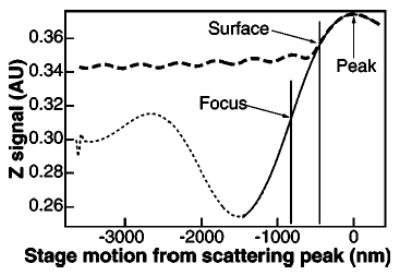
Axial position signals for a free (heavy dashed line) and stuck (light dashed line) bead as the stage was scanned in the axial direction. All stage motion is relative to the scattering peak, which is indicated on the right of the figure. The positions of the surface (measured) and the focus [calculated from Eq. (5)] are indicated by vertical lines. The axial detection fit [Eq. (5)] to the stuck bead trace is shown in the region around the focus as a heavy solid line.

FIG. 9

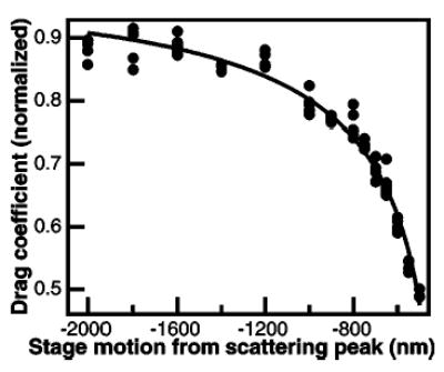
Normalized drag coefficient (β₀/β, where β₀ is the Stokes drag on the sphere: 6πηa) as a function of distance from the scattering peak. The normalized inverse drag coefficient (solid circles) was determined through rolloff measurements and from the displacement of a trapped bead as the stage was oscillated. The normalized inverse drag coefficient was fit to Faxen’s law [Eq. (6)] with a height offset ɛ and scaling parameter δ, which is the fractional focal shift, as the only free parameters: β_0/β =1−(9/16)×[aδ⁻¹(z−ɛ)⁻¹] + 1/8[aδ⁻¹(z−ɛ)⁻¹]³−(45/256)[aδ⁻¹(z−ɛ)⁻¹]⁴−(1/16)[aδ⁻¹(z−ɛ)⁻¹]⁵, where a is the bead radius, z is the motion of the stage relative to the scattering peak, β₀ is the Stoke’s drag on the bead, (6πηa), and β is the measured drag coefficient. The fit returned a fractional focal shift δ of 0.82±0.02 and an offset ɛ of 161 nm. The position of the surface relative to the scattering peak is obtained by setting the position of the bead center, δ(z−ɛ) equal to the bead radius a, which returns a stage position of 466 nm above the scattering peak, as indicated in Fig. 8.

FIG. 10

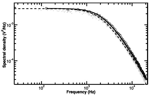
Power spectrum of a trapped bead. Power spectrum of a 0.5 μm polystyrene bead trapped 1.2 μm above the surface of the trapping chamber recorded with a PSD (gray dots). The raw power spectrum was averaged over 256 Hz windows on the frequency axis (black circles) and fit (black line) to a Lorentzian [Eq. (7)] corrected for the effects of the antialiasing filter, frequency dependent hydrodynamic effects, and finite sampling frequency, as described by Berg–Sørensen and Flyvbjerg (Ref. 148). The rolloff frequency is 2.43 kHz, corresponding to a stiffness of 0.08 pN/nm. For comparison the raw power spectrum was fit to an uncorrected Lorentzian (dashed line), which returns a rolloff frequency of 2.17 kHz. Whereas the discrepancies are on the order 10% for a relatively weak trap, they generally become more important at higher rolloff frequencies.

FIG. 11

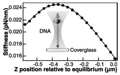
Axial dependence of lateral stiffness. The experimental geometry for these measurements is depicted in the inset. A polystyrene bead is tethered to the surface of the cover glass through a long DNA tether. The stage was moved in the negative z direction (axial), which pulls the bead towards the laser focus, and the lateral stiffness was determined by measuring the lateral variance of the bead. The data (solid circles) are fit with the expression for a simple dipole [Eq. (14)], with the power in the specimen plane, the beam waist, and an axial offset as free parameters.

FIG. 12

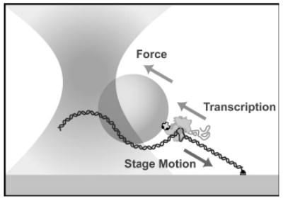
Cartoon of the experimental geometry (not to scale) for single-molecule transcription experiment. Transcribing RNA polymerase with nascent RNA (gray strand) is attached to a polystyrene bead. The upstream end of the duplex DNA (black strands) is attached to the surface of a flowchamber mounted on a piezoelectric stage. The bead is held in the optical trap at a predetermined position from the trap center, which results in a restoring force exerted on the bead. During transcription, the position of the bead in the optical trap and hence the applied force is maintained by moving the stage both horizontally and vertically to compensate for motion of the polymerase molecule along the DNA (adapted from Ref. 87).

FIG. 13

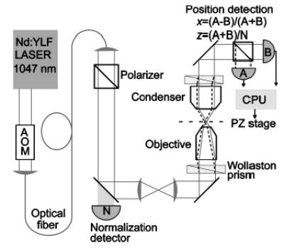
The optical trapping interferometer. Light from a Nd:YLF laser passes through an acoustic optical modulator (AOM), used to adjust the intensity, and is then coupled into a single-mode polarization-maintaining optical fiber. Output from the fiber passes through a polarizer to ensure a single polarization, through a 1:1 telescope and into the microscope where it passes through the Wollaston prism and is focused in the specimen plane. The scattered and unscattered light is collected by the condenser, is recombined in the second Wollaston prism, then the two polarizations are split in a polarizing beamsplitter and detected by photodiodes A and B. The bleedthrough on a turning mirror is measured by a photodiode (N) to record the instantaneous intensity of the laser. The signals from the detector photodiodes and the normalization diode are digitized and saved to disk. The normalized difference between the two detectors (A and B) gives the lateral, x displacement, while the sum signal (A+B) normalized by the total intensity (N) gives the axial, z displacement.

FIG. 14

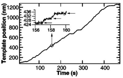
Two-dimensional, stage based force clamp. Position record of a single RNA polymerase molecule transcribing a 3.5 kbp (1183 nm) DNA template under 18 pN of load. The x and z position signals were low pass filtered at 1 kHz, digitized at 2 kHz, and boxcar averaged over 40 points to generate the 50 Hz feedback signals that controlled the motion of the piezoelectric stage. Motion of the stage was corrected for the elastic compliance of the DNA (Ref. 39) to recover the time-dependent contour length, which reflects the position of the RNA polymerase on the template. Periods of roughly constant velocity are interrupted by pauses on multiple timescales. Distinct pauses can be seen in the trace, while shorter pauses (~1 s) can be discerned in the expanded region of the trace (inset: arrows).