Effects of sensing behavior on a latency code

Abstract

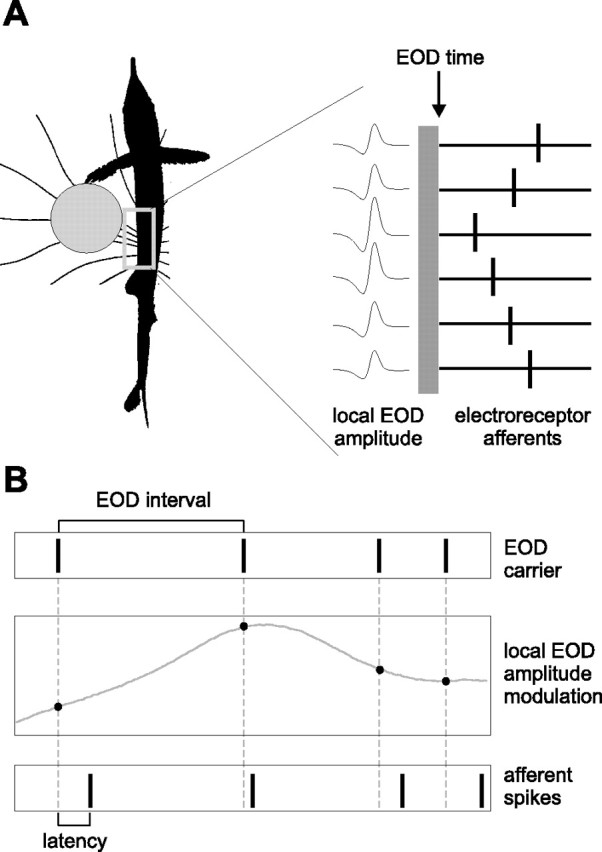
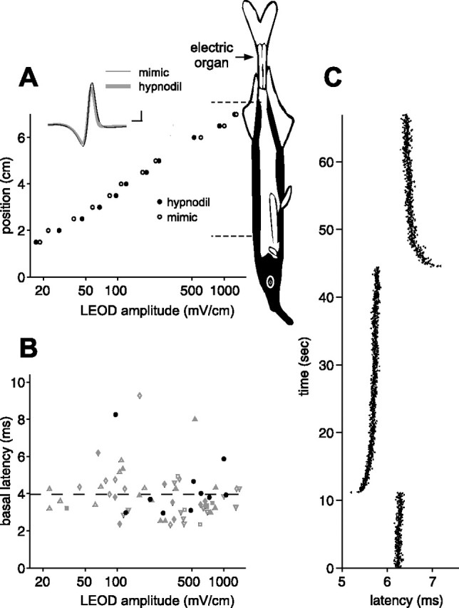
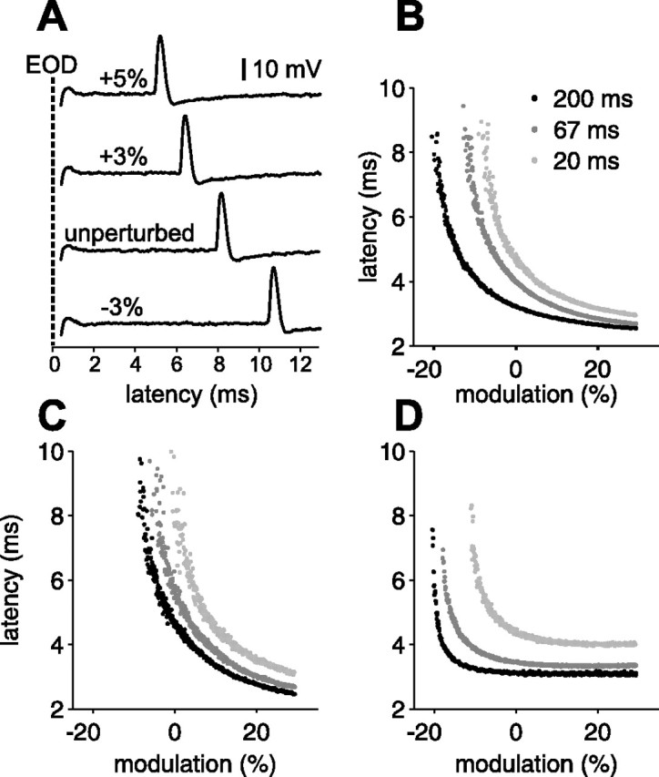
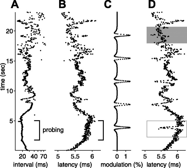
Sensory information is often acquired through active exploration, yet relatively little is known about how neurons encode sensory stimuli in the context of natural patterns of sensing behavior. We examined the effects of sensing behavior on a spike latency code in the active electrosensory system of mormyrid fish. These fish actively probe their environment by emitting brief electric organ discharge (EOD) pulses. Nearby objects alter the spatial pattern of current flowing through the skin. These changes are encoded by small shifts in the latency of individual electroreceptor afferent spikes after the EOD. In nature, the temporal pattern of EOD intervals is highly structured and varies depending on the behavioral context. We performed experiments in which we varied both the EOD amplitude and the intervals between EODs to understand how sensing behavior affects afferent latency coding. We use white-noise stimuli and linear filter estimation methods to develop simple models characterizing the dependence of afferent spike latency on the preceding sequence of EOD intervals and amplitudes. Comparing the predictions of these models with actual afferent responses for natural patterns of EOD intervals and amplitudes reveals an unexpectedly rich interplay between sensing behavior and stimulus encoding. Implications of our results for how afferent spike latency is decoded at central stages of electrosensory processing are discussed.

Figure 1.

Spatial and temporal aspects of latency coding in the mormyrid electrosensory system. A, A nearby conductive object alters the pattern of current flowing through the fish’s skin at the time of the EOD (left). Object-induced changes in the LEOD amplitude are encoded by the latencies of spikes in afferents innervating neighboring electroreceptors (right). LEOD amplitude is larger for electroreceptor afferents closest to the object, resulting in shorter spike latencies. B, Pulse-type mormyrid fish emit brief EOD pulses separated by much longer intervals (top). External stimuli result in modulations in EOD amplitude sampled at the time of the EOD pulses (middle). At each electroreceptor, sequences of EOD amplitudes are encoded by sequences of afferent spike latencies (bottom).

Figure 2.

Afferent spike latency adapts to the mean EOD amplitude. A, Comparison of LEOD amplitudes measured near the skin of the fish at different rostrocaudal positions (aligned with schematic of fish). LEODs resulting from the fish’s natural discharge were similar to those resulting from our mimic. Representative LEOD waveforms are shown in the inset. Calibration: 100 mV/cm, 0.1 ms. Schematic of the fish indicates the location of the electric organ and the regions of the skin containing electroreceptors (black). Dashed lines indicate the area of the skin innervated by afferents of the posterior lateral line nerve recorded in this study. B, Differences in baseline first spike latencies in response to the EOD mimic are uncorrelated with LEOD amplitude at the receptor. Each point represents a single afferent, and different symbols represent afferents from different fish. Black circles represent afferents recorded in a naturally discharging fish. C, Adaptation in afferent first spike latency to an abrupt 5% increase followed by an abrupt 5% decrease in EOD amplitude. EOD interval was held constant at 33 ms. Note that adaptation is initially rapid and then proceeds at a much slower rate.

Figure 3.

Afferent spike latency depends on EOD amplitude and sensing behavior. A, Representative extracellular traces illustrating the shift in afferent spike latency resulting from changes in EOD amplitude. The interval between EODs was 67 ms. B–D, Smooth ramps in EOD amplitude at three constant EOD intervals (200, 67, and 20 ms) for three different afferents. Increases in EOD amplitude result in smooth decreases in afferent first spike latency. The shorter the EOD interval, the longer the latency for a given amplitude.

Figure 4.

Effects of natural sensing intervals on afferent spike latency. A, EOD intervals recorded in a behavioral experiment in which a fish discriminated between two objects and then foraged for food. Intervals were short and regular during probing (bracket) and longer and irregular during foraging. B, Afferent first spike latency evoked by a constant EOD amplitude delivered at the natural EOD intervals shown in A. Latency clearly depends on the previous intervals, increasing as EOD interval decreases. D, Latency shifts evoked by small transient increases in EOD amplitude (shown in C) are clear when sensing interval is approximately constant (open rectangle) but can be obscured when sensing intervals vary (shaded rectangle). EOD intervals are the same as shown in A.

Figure 5.

Subsequent spikes in the afferent response do not carry additional information. A, Mean second spike latency versus mean first spike latency for a putative A-type afferent. Each point is based on responses to a different stretch of random EOD amplitudes and sensing intervals. Error bars are SEMs. B, Mean second and third spike latency (black and gray, respectively) versus mean first spike latency for a putative B-type afferent. In both A and B, subsequent spike latencies appear to be simple functions of (i.e., are correlated with) first spike latency.

Figure 6.

Approximate linear summation of effects of previous EOD intervals and present EOD amplitude. A, Histogram of latencies for the following (top to bottom): no previous EOD within 80 ms (baseline); one previous EOD, 17–32 ms before the present (1); one previous EOD, 32–47 ms before the present (2); and two previous EODs, one 17–32 ms before the present and one 32–47 ms before the present (both). Mean latency indicated by vertical line. B, Change in mean latency from baseline, for conditions 1, 2, and both, and the linear sum of 1 and 2 (sum). Error bars are SEMs. C, Histogram of latencies for the following (top to bottom): no previous EOD within 80 ms (baseline); present EOD amplitude larger than the mean (0.1–0.5% modulation) (1); one previous EOD, 17–32 ms before the present (2); and present EOD larger than the mean and one previous EOD, 17–32 ms before the present (both). D, Change in mean latency from baseline, for conditions 1, 2, and both, and the linear sum of 1 and 2 (sum). Data in A–D are from a representative afferent. E, Linearity ratios (see Results) for the effects of two previous EODs for 18 afferents. F, Linearity ratios for the effects of present EOD amplitude and previous EOD for the same afferents as in E, excluding those for which the effects of 1, 2, or sum were not statistically significant (p > 0.05). Gray lines indicate ±10% deviation from linearity, and dashed lines indicate ±20% deviation from linearity.

Figure 7.

Relative contributions of EOD amplitude and sensing intervals to afferent output revealed by a linear filter analysis. A, Schematic illustrating input to the electrosensory system as a carrier plus modulations. The temporal characteristics of the carrier are not fixed as the sequence of EOD intervals varies. B, F, Carrier and modulation filters for first spike latency for two different afferents, computed from experiments in which EODs were delivered at independent intervals (17–100 ms) with independent Gaussian amplitude modulation SDs of 1% (B) and 5% (F) of the unperturbed EOD amplitude. Sensitivity to present EOD amplitude modulation is indicated by the black circle. Sensitivity to past amplitude modulations is indicated by the black curve. Sensitivity to previous intervals is indicated by the gray curve. Aggregate sensitivity to all previous intervals is indicated by gray circle. Filters are not defined in gray region in which no EODs occur. E, Static nonlinearity mapping filter output onto predicted latency, for the afferent in F. C, G, Actual first spike latency versus latency predicted by the linear filters in B and F. D, H, Actual versus predicted first spike latency based on the present EOD amplitude alone.

Figure 8.

Collective data for white-noise filters. A, Overlay of carrier filters for all afferents tested. Inset, Carrier filters show roughly exponential decay. B, Overlay of modulation filters for past modulations for all afferents tested. C, Histogram of aggregate interval sensitivities. D, Histogram of present amplitude sensitivities. E, Coefficient of determination (r²) between actual and predicted first spike latency versus size of amplitude modulation. F, Relative importance of the present EOD amplitude (ratio of r² for the prediction using present EOD alone to that for the prediction using present and past) versus size of modulation amplitude. For modulation SDs of ∼1–2% of the unperturbed EOD amplitude, present and past are comparable in importance.

Figure 9.

White-noise filters are partially successful in predicting response for natural EOD intervals. A, For 11 afferents, coefficient of determination between actual latency and latency predicted by white-noise filters, for independent intervals and independent amplitude modulations (*), for natural intervals and independent amplitude modulations (+), and for natural intervals and correlated (low-pass filtered at 1Hz) amplitude modulations (□). Gray symbols indicate filters augmented with a static nonlinearity. Prediction accuracy is lower for natural intervals and for correlated amplitude modulations. The natural interval sequence used in these experiments is shown in Figure 4A. B–D, Actual versus predicted latency in an example afferent, for independent intervals and independent amplitudes (B), natural intervals and independent amplitudes (C), and natural intervals and correlated amplitudes (D).

Figure 10.

Discrepancies between actual and predicted latency for natural intervals and correlated amplitudes suggest a relationship between sensing rate, frequency of amplitude modulation, and afferent gain. A, B, Predicted (A) and actual (B) latency versus modulation amplitude, for natural intervals and independent amplitudes, with points colored by instantaneous rate. Actual latency has greater amplitude gain (magnitude of slope) at higher rates (red), whereas predicted latency has roughly constant gain. C, D, Same as A and B, but for correlated amplitudes. Actual latency (D) shows roughly constant amplitude gain at different rates, whereas predicted latency (C) shows markedly lower gain at high rates. E, F, Normalized gain versus cutoff frequency of correlated amplitude modulations (1 Hz, 7.5 Hz) at low EOD rate (blue) or high EOD rate (red), for predicted latency (E) and actual latency (F), in 11 afferents. Gains are normalized by gain for independent (ind) modulations in the same afferent. For plotting purposes, ind is placed at 30 Hz, just above the Nyquist frequency for EOD intervals used. G, Schematic explanation for the loss of gain in predicted latency in C. If the correlation time of amplitude modulations is much greater than the filter width, then modulation amplitude is roughly constant over the filter window. Present and past modulation amplitudes then make opposing contributions to latency. The summed effects of past and present modulations at low rate (blue circles) lead to a small loss of gain, but, at high rate (red circles), the loss may be substantial. Values for the respective gains are indicated by dashed lines. H, Calculated gain versus low-pass cutoff frequency of correlated amplitude modulations, for constant rates of 17 (mean rate for white-noise protocol), 25, 35, and 50 Hz, using the white-noise modulation filter for the afferent shown in A–D. Longer correlation times (lower cutoff frequencies) lead to a loss of gain at all rates, but the loss is greater at higher rates.

Figure 11.

Sensitivity to present EOD amplitude increases linearly with constant EOD rate. A, B, Actual latency versus present EOD modulation amplitude for two afferents, at constant EOD rates of 15 Hz (blue), 30 Hz (purple), and 50 Hz (red), for independent amplitude modulations. Note the steeper slope (gain) at higher rates. C, D, Modulation filters for the afferents in A and B, for these three constant intervals. Modulation filters for independent intervals for the same afferents are shown in black. Sensitivity to present amplitude modulation (circles at time 0) increases approximately linearly (insets) with increasing rate. Gray line in insets is a least-squares fit to the three constant-interval sensitivities. E, Calculated gain versus low-pass cutoff frequency of correlated amplitude modulations, for the white-noise modulation filter of the afferent in A and C with present amplitude sensitivity scaled according to the relationship in C, inset. Longer correlation times (lower cutoff frequencies) still lead to a loss of gain at all rates, but the loss at higher rates is no worse than at lower rates; compare with Figure 10H, which is based on the white-noise filter for the same afferent. F, A portion of the protocol used for the afferent in B. Note the longer mean latencies at higher rates, with both rapid and slower phases of drift after a change in rate. Only the second half of each constant-rate block was used for analysis.

Figure 12.

White-noise filter predictions for natural intervals and correlated amplitudes can be substantially improved by incorporating interval-dependent amplitude sensitivity changes. A, Natural interval sequence recorded in a behavioral experiment. B, Independent amplitude modulations low-pass filtered at 1 Hz and sampled at the EOD times in A. C, Actual latency (black) and latency predicted by white-noise filters (blue) for the intervals and amplitudes shown in A and B, respectively. D, Actual latency (black) and latency predicted by white-noise filters (pink) incorporating both a constant shift and a scaling of sensitivity to present modulation amplitude by an amount proportional to the mean rate over the previous 3 s. E, Actual latency versus prediction from scaled filters; corresponding plot for unscaled filters is shown in Figure 9D. F, For five afferents, coefficient of determination between actual latency and latency predicted by white-noise filters on independent intervals and independent amplitudes (*), by white-noise filters on natural intervals and correlated amplitudes (blue square), and by scaled white-noise filters on natural intervals and correlated amplitudes (pink square). Interval-dependent scaling of sensitivity to present modulation amplitude increases prediction accuracy in all five afferents.

References

1. Attneave F (1954). Some informational aspects of visual perception. Psychol Rev 61:183–193. - PubMed
1. Barlow H (1961). Possible principles underlying the transformation of sensory messages. In: In: Sensory communication (Rosenblith W, ed.) pp. 217–234. Cambridge, MA: MIT.
1. Bell CC (1990a). Mormyromast electroreceptor organs and their afferents in mormyrid electric fish. II. Intra-axonal recordings show initial stages of central processing. J Neurophysiol 63:303–318. - PubMed
1. Bell CC (1990b). Mormyromast electroreceptor organs and their afferents in mormyrid electric fish. III. Physiological differences between two morphological types of fibers. J Neurophysiol 63:319–332. - PubMed
1. Bell CC, Russell CJ (1978). Termination of electroreceptor and mechanical lateral line afferents in the mormyrid acousticolateral area. J Comp Neurol 182:367–382. - PubMed
Publication types