Climate cycles and forecasts of cutaneous leishmaniasis, a nonstationary vector-borne disease

Abstract

Background: Cutaneous leishmaniasis (CL) is one of the main emergent diseases in the Americas. As in other vector-transmitted diseases, its transmission is sensitive to the physical environment, but no study has addressed the nonstationary nature of such relationships or the interannual patterns of cycling of the disease.

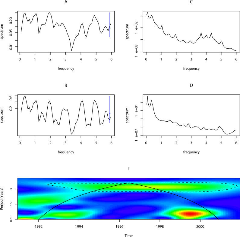
Methods and findings: We studied monthly data, spanning from 1991 to 2001, of CL incidence in Costa Rica using several approaches for nonstationary time series analysis in order to ensure robustness in the description of CL's cycles. Interannual cycles of the disease and the association of these cycles to climate variables were described using frequency and time-frequency techniques for time series analysis. We fitted linear models to the data using climatic predictors, and tested forecasting accuracy for several intervals of time. Forecasts were evaluated using "out of fit" data (i.e., data not used to fit the models). We showed that CL has cycles of approximately 3 y that are coherent with those of temperature and El Niño Southern Oscillation indices (Sea Surface Temperature 4 and Multivariate ENSO Index).

Conclusions: Linear models using temperature and MEI can predict satisfactorily CL incidence dynamics up to 12 mo ahead, with an accuracy that varies from 72% to 77% depending on prediction time. They clearly outperform simpler models with no climate predictors, a finding that further supports a dynamical link between the disease and climate.

Figure 1. Time Series

(A) CL cases in Costa Rica. (B) Mean temperature in Costa Rica. (C) SST 4. (D) MEI. (E) Box plot with monthly square-root-transformed CL cases. (F) The fits of (1) the Daubechies discrete wavelet (green lines), used to detrend the series so that the resulting data can then be analyzed for their dominant frequencies with a periodogram (a filter number 5 and eight levels of decomposition were used for this wavelet; the dashed line corresponds to periodic edges, and the dotted line to symmetric ones); (2) smoothing splines (blue solid line) and the first four reconstructed components of singular spectrum analysis (black dashed line; 60 orders). These methods were used to de-noise the signals so that dominant frequencies could be identified (with the maximum entropy spectral density method).

Figure 2. Dominant Frequencies in the Data

(A and B) Smoothed periodograms for (A) the detrended series (using Daubechies discrete wavelet with filter number 5 and periodic edges) and (B) the detrended series (using Daubechies discrete wavelet with filter number 5 and symmetric edges). In the periodograms, the blue lines are the 95% point confidence intervals [19]. (C and D) Maximum entropy spectral density for (C) the de-noised series (with smoothing splines) and (D) the de-noised series (with singular spectrum analysis). For the periodograms and the maximum entropy spectral density, frequencies are in cycles per year. (E) Wavelet power spectrum. The solid line is the cone of influence indicating the region of time and frequency where the results are not influenced by the edges of the data and are therefore reliable. The dashed line corresponds to the 95% confidence interval for white noise based on the variance of the square-root-transformed incidence series. The intervals were obtained using a chi-squared distributed statistic with one degree of freedom (see [22] for details). The Morlet wavelet was used [18,21,22]. In all analyses, the cases are square-root-transformed. Maximum entropy spectral densities were computed using the software described in [20]. For the maximum entropy spectral density an autoregressive process of order p = 40 was used, i.e., AR(40).

Figure 3. Cross-Wavelet Coherency and Phase

The coherency scale is from zero (blue) to one (red). Thus, red regions indicate frequencies and times for which the two series share variability. The cone of influence (within which results are not influenced by the edges of the data) and the significant (p < 0.05) coherent time-frequency regions are indicated by solid lines. The colors in the phase plots correspond to different lags between the variability in the two series for a given time and frequency, measured in angles from −PI to PI. A value of PI corresponds to a lag of 16 mo. Cases are square-root-transformed. The procedures and software are those described in [21]. A smoothing window of 15 mo (2w + 1 = 31) was used to compute the cross-wavelet coherence.

Figure 4. Cross-Correlation Functions of Square-Root-Transformed Cases with SST 4, Temperature, and MEI

(A–C) Cross-correlation functions (CCF) with (A) SST 4, (B) MEI, (C) Temperature. The blue dashed lines are the 95% point confidence intervals for the cross-correlation between two series that are white noise [23]. (D) Predictive R ² measuring the accuracy of the predictions. Blue is for predictions with only 9 y of training data (used to fit the model) and black for predictions generated with all months preceding the prediction. (The value for 12-mo predictions with temperature is not shown, because it was negative.)

References

1. Gratz NG. Emerging and resurging vector borne diseases. Annu Rev Entomol. 1999;44:e380 - PubMed
1. Lainson R, Shaw JJ. Epidemiology and ecology of leishmaniasis in Latin-America. Nature. 1978;273:595–600. - PubMed
1. Chaves LF, Hernandez MJ. Mathematical modelling of American cutaneous leishmaniasis: Incidental hosts and threshold conditions for infection persistence. Acta Trop. 2004;92:245–252. - PubMed
1. Silveira FT, Lainson R, Corbett CE. Clinical and immunopathological spectrum of American cutaneous leishmaniasis with special reference to the disease in Amazonian Brazil—A review. Mem Inst Oswaldo Cruz. 2004;99:231–251. - PubMed
1. Zeledon R. Cutaneous leishmaniais and Leishmania infantum . Trans R Soc Trop Med Hyg. 1991;85:557. - PubMed
Publication types