. 2006 Aug 30;26(35):9030-7.
doi: 10.1523/JNEUROSCI.0225-06.2006.

Decoding stimulus variance from a distributional neural code of interspike intervals

Affiliations

Decoding stimulus variance from a distributional neural code of interspike intervals

Brian Nils Lundstrom et al. J Neurosci. .

Abstract

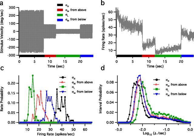
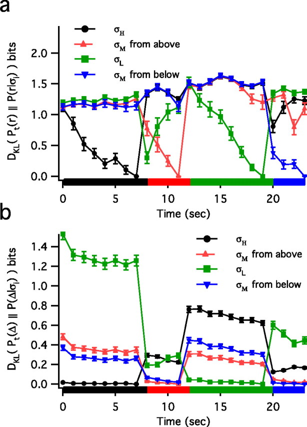
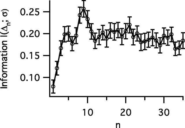
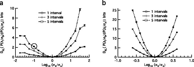
The spiking output of an individual neuron can represent information about the stimulus via mean rate, absolute spike time, and the time intervals between spikes. Here we discuss a distinct form of information representation, the local distribution of spike intervals, and show that the time-varying distribution of interspike intervals (ISIs) can represent parameters of the statistical context of stimuli. For many sensory neural systems the mapping between the stimulus input and spiking output is not fixed but, rather, depends on the statistical properties of the stimulus, potentially leading to ambiguity. We have shown previously that for the adaptive neural code of the fly H1, a motion-sensitive neuron in the fly visual system, information about the overall variance of the signal is obtainable from the ISI distribution. We now demonstrate the decoding of information about variance and show that a distributional code of ISIs can resolve ambiguities introduced by slow spike frequency adaptation. We examine the precision of this distributional code for the representation of stimulus variance in the H1 neuron as well as in the Hodgkin-Huxley model neuron. We find that the accuracy of the decoding depends on the shapes of the ISI distributions and the speed with which they adapt to new stimulus variances.


Figures

Figure 1.
Figure 1.
Ambiguity in the rate with respect to the stimulus SD is reduced by considering spike intervals. a, A schematic of the velocity stimulus to the fly. This three-state 24 s stimulus was repeated for 2 h. Stimulus SDs were σH = 3σM = 9σL. b, Mean spike rate for the three-state switching experiment with bin size of 10 ms. c, Rate distributions P(ri) from the last second of each epoch. d, ISI distributions P(Δ|σi) from the last second of each epoch. Note that stimuli with σM lead to two distinct rate distributions (c, triangles) but very similar ISI distributions (d, triangles).
Figure 2.
Figure 2.
Kullback–Leibler divergence DKL between the time-dependent distributions and the relevant reference distributions for rate DKL [Pt(r),P(ri)] (a) and intervals DKL [Pt(Δ),P(Δ|σi)] (b). Each distribution was created from 1 s (times 300 repeats) of this 24 s stimulus pattern. Reference distributions are sampled from the final second of each of the four epochs, hence DKL = 0 at 7, 11, 19, and 23 s. Although rate distributions change continuously throughout the epoch (a), interval distributions quickly reach a steady state (b). Error bars represent the SD.
Figure 3.
Figure 3.
The information In;σ) gained from successive spikes after a switch between SDs as calculated by Equation 4. The probability Pni) of a given interval value for the nth interval after an SD switch is calculated for each of the three σ values in Figure 1. After approximately three intervals, the information per spike reaches steady state, suggesting that interval coding quickly adapts to the new stimulus statistics. Error bars represent the SD.
Figure 4.
Figure 4.
Calculating the difference between different steady-state ISI distributions. Displayed are log–ISI distributions in response to zero-mean random stimuli from fly H1 neuron (a) and HH model neuron (b) in which stimulus SDs (normalized to the lowest SD) are shown in the figure key (right) and the mean firing rates (Hz) are shown in parentheses. Bin width is 0.05 log10 units; the sum of all bins equals one. Shown also are contours of the Kullback–Leibler divergence DKL between the log–ISI distributions for the fly H1 neuron (c) and HH model neuron (d) as calculated from Equation 1. In the fly there is generally a larger difference between the distributions for the transition from a low-variance to high-variance condition, i.e., for σA < σB, rather than vice versa. The model neuron shows the opposite trend. The distributions corresponding to the three smallest stimulus SD values for the HH model neuron shown in b are omitted from additional analyses.
Figure 5.
Figure 5.
Cumulative Kullback–Leibler divergence (DcKL(n)) between neural responses, as defined in Equation 2, as a function of the log ratio of two stimulus SDs, σB and σA. This divergence is related to the probability of misclassification in which a distance of one bit corresponds to a twofold reduction in error and is a measure of the capacity to discriminate between two ISI distributions resulting from two stimulus variances, as in Figure 4, a and b. DcKL(n) is for n = 1, 3, or 5 ISIs from fly data for a given SD ratio (a) and from the HH model neuron (b). For example, the circle represents the average discrimination for all 10-fold ratios of stimulus SD decrease, e.g., 10 to 1, 30 to 3, and 60 to 6. Error bars represent the SD.
Figure 6.
Figure 6.
Number of spikes and corresponding mean time needed for discrimination, where discrimination is defined as a distance of one bit. For each data series, the stimulus SD of the comparison distribution (σA) is held constant while the SD of the source distribution varies (σB). a, Number of H1 spikes required to discriminate between two variances. b, HH spikes required to discriminate between two variances. c, Mean time (seconds) in fly H1 neuron required to discriminate between two variances. d, Mean time (seconds) in HH neuron required to discriminate between two variances. Discrimination requires considerably fewer spikes and less time in the model neuron as compared with the fly neuron. The figure key values (right) for σA and σB are in normalized units of SD, which correspond to those in Figure 4.
Figure 7.
Figure 7.
Testing the independence assumption. a, Kullback–Leibler divergences calculated by using independent distributions for P1|σ) and P2|σ) (triangles) and joint distributions P12|σ) (circles) as a function of the log ratio of two stimulus SDs, σB and σA, for independent distributions; error bars represent the SD. b, Mutual information, Equation 5, between the first spike interval and the nth interval of fly data for interval sequences that result from steady-state zero-mean stimuli with varying SDs. The sharp decrease between n = 2 and n = 3 suggests that dependence between intervals is confined mainly to the first and second interval; other intervals effectively are drawn randomly from the probability distribution. This information calculation was corrected for undersampling, as described in Materials and Methods. Gray lines represent the mutual information between intervals from different variance distributions, whereas the black line represents the mean; error bars represent the SD across different stimulus conditions.
Figure 8.
Figure 8.
Decoding a time-varying stimulus SD from HH spike trains by using 2 ISIs (a) and 15 ISIs (b, green lines). For each data point we find σ, for which Pn|σ) is maximized for either 2 or 15 intervals, as in Equation 6. Stimulus SD is estimated from the rate calculated in a window width equal to the mean time of 2 or 15 intervals (22 and 314 ms, respectively; red circles). The instantaneous stimulus SD is shown in black. At very short times, the range of possible estimates is limited when calculated from rate, but not from intervals. For longer times, the estimates from rate and intervals are comparable, because the HH model does not show slow spike frequency and would not be expected to display the ambiguity between rate and intervals as in fly neuron (Fig. 1). Shown is a comparison of estimated versus true SD, using intervals (c) and spike rate (d), in which the vertical bars represent the SDs of the estimated SD, and mean-squared error of the estimated SD (e) as a function of interval number or spike rate bin width.

Similar articles

Cited by

References

    1. Baccus SA, Meister M. Fast and slow contrast adaptation in retinal circuitry. Neuron. 2002;36:909–919. - PubMed
    1. Bialek W, Rieke F, de Ruyter van Steveninck RR, Warland D. Reading a neural code. Science. 1991;252:1854–1857. - PubMed
    1. Brenner N, Strong SP, Koberle R, Bialek W, de Ruyter van Steveninck RR. Synergy in a neural code. Neural Comput. 2000;12:1531–1552. - PubMed
    1. Carandini M, Ferster D. A tonic hyperpolarization underlying contrast adaptation in cat visual cortex. Science. 1997;276:949–952. - PubMed
    1. Cariani P. Temporal coding of periodicity pitch in the auditory system: an overview. Neural Plast. 1999;6:147–172. - PMC - PubMed

Publication types

LinkOut - more resources