The gap effect is exaggerated in parafovea

Abstract

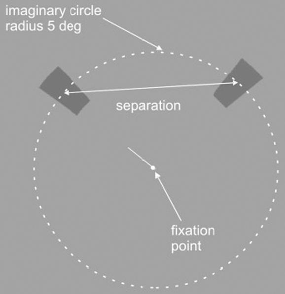
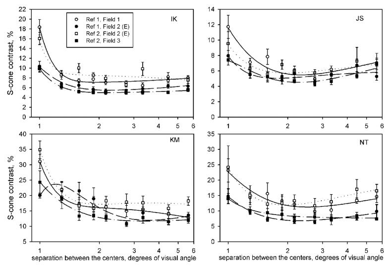
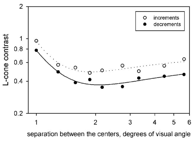
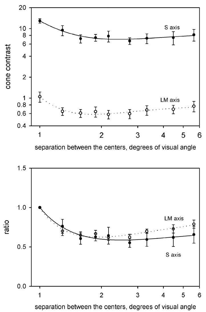
In central vision, the discrimination of colors lying on a tritan line is improved if a small gap is introduced between the two stimulus fields. Boynton et al. (1977) called this a "positive gap effect." They found that the effect was weak or absent for discriminations based on the ratio of the signals of long-wave and middle-wave cones; and even for tritan stimuli, the gap effect was weakened when forced choice or brief durations were used. We here describe measurements of the gap effect in the parafovea. The stimuli were 1 deg of visual angle in width and were centered on an imaginary circle of radius 5 deg. They were brief (100 ms), and thresholds were measured with a spatial two-alternative forced choice. Under these conditions we find a clear gap effect, which is of similar magnitude for both the cardinal chromatic axes. It may be a chromatic analog of the crowding effect observed for parafoveal perception of form.

Fig. 1

A black-and-white example of the stimuli used in the experiments. The centers of the two stimulus patches lie on an imaginary circle indicated by the broken line. One stimulus, chosen at random, is the referent stimulus, and the other is the test or variable stimulus. The separation of the two stimuli is expressed as the distance between their centers in degrees of visual angle. The radial length of each stimulus sector is 2 deg, and its width at its midpoint is 1 deg. A central fixation point is continuously present. A thin bar marker, concurrent with the test and referent stimuli, points to the more clockwise of the two.

Fig. 2

Chromaticity diagram representing the referent stimuli and the backgrounds. The diagram is an analog of the standard MacLeod-Boynton diagram but is constructed from the 10-deg Stockman-Sharpe (2000) fundamentals. The left-hand panel shows the locations of the referent and background values for Experiment 1 (discrimination on the S axis), while the right-hand panel shows the corresponding values for Experiment 2 (discrimination on the L/M axis). G and R denote the chromaticities of the green and red phosphors of the monitor, and the solid lines delimit the gamut of the possible colors that the monitor can produce.

Fig. 3

Individual results for Experiment 1 (discrimination on the S axis). The four panels show results for individual observers. The abscissa in each case shows the spatial separation between the centers of referent and test stimuli, expressed on a logarithmic scale. When the separation of the midpoints is 1 deg, the edges of the stimuli are abutting. The ordinate shows the threshold as a percentage change in the S-cone signal. The error bars represent ±1 SEM and are based on between-session variance. The four data sets in each panel correspond to the four combinations of referent and background chromaticity (see legend and Fig. 2). The fitted smooth curves are inverse third-order polynomials and are not intended to have theoretical significance.

Fig. 4

Average results for incremental and decremental targets in Experiment 1 (discrimination on the S axis). Data have been averaged across the four observers. The abscissa shows the spatial separation between the centers of referent and test stimuli, expressed on a logarithmic scale, and the ordinate shows the log S-cone contrast at threshold. The error bars represent ±1 SEM and are based on intersubject variance; their size reflects the absolute differences between subjects' thresholds. The curves fitted to the data points are inverse third-order polynomials and are not intended to have theoretical significance.

Fig. 5

Individual results for Experiment 2 (discrimination on the L/M axis). The two panels show results for individual observers. The abscissa in each case shows the spatial separation between the centers of referent and test stimuli, expressed on a logarithmic scale. The ordinate shows the threshold as a percentage change in the L-cone signal. The error bars represent ±1 SEM and are based on between-session variance. The four data sets in each panel correspond to the four combinations of referent and background chromaticity (see legend and Fig. 2). The fitted smooth curves are inverse third-order polynomials and are not intended to have theoretical significance.

Fig. 6

Average results for incremental and decremental targets in Experiment 2 (discrimination on the L/M axis). The plots show data averaged across observers. The abscissa shows the spatial separation between the centers of referent and test stimuli, expressed on a logarithmic scale, and the ordinate shows the log L-cone contrast at threshold. The smooth curves fitted to the data points are inverse third-order polynomials and are not intended to have theoretical significance.

Fig. 7

Results for Experiment 3 (ounterbalanced comparison of discriminations on the two cardinal axes). The upper panel shows the thresholds for S and for L/M axes, expressed on a logarithmic scale in order to accommodate the differences in absolute sensitivity. In the lower panel, to allow a direct comparison of the relative shapes of the functions for the two axes, thresholds are reexpressed as a ratio of the threshold when the edges of the sectors are abutting. The error bars represent ±1 SEM and are based on intersubject variance. The smooth curves fitted to the data points are inverse third-order polynomials and are not intended to have theoretical significance.

Fig. 8

Mean response times in Experiment 3. The error bars represent ±1 SEM and are based on intersubject variance. The smooth curves fitted to the data points are inverse third-order polynomials and are not intended to have theoretical significance.

References

1. Bouma H. Interaction effects in parafoveal letter recognition. Nature. 1970;226:177–178. - PubMed
1. Boynton RM, Hayhoe MM, MacLeod DIA. The gap effect: Chromatic and achromatic visual discrimination as affected by field separation. Optica Acta. 1977;24:159–177.
1. Brindley GS. The summation areas of human colour-receptive mechanisms at increment threshold. Journal of Physiology. 1954;124:400–408. - PMC - PubMed
1. Cottaris NP, De Valois RL. Temporal dynamics of chromatic tuning in macaque primary visual cortex. Nature. 1998;395:896–900. - PubMed
1. Dacey DM, Lee BB. The “blue-on” opponent pathway in primate retina originates from a distinct bistratified ganglion cell type. Nature. 1994;367:731–735. - PubMed
Publication types