Forced and unforced ocean temperature changes in Atlantic and Pacific tropical cyclogenesis regions

Abstract

Previous research has identified links between changes in sea surface temperature (SST) and hurricane intensity. We use climate models to study the possible causes of SST changes in Atlantic and Pacific tropical cyclogenesis regions. The observed SST increases in these regions range from 0.32 degrees C to 0.67 degrees C over the 20th century. The 22 climate models examined here suggest that century-timescale SST changes of this magnitude cannot be explained solely by unforced variability of the climate system. We employ model simulations of natural internal variability to make probabilistic estimates of the contribution of external forcing to observed SST changes. For the period 1906-2005, we find an 84% chance that external forcing explains at least 67% of observed SST increases in the two tropical cyclogenesis regions. Model "20th-century" simulations, with external forcing by combined anthropogenic and natural factors, are generally capable of replicating observed SST increases. In experiments in which forcing factors are varied individually rather than jointly, human-caused changes in greenhouse gases are the main driver of the 20th-century SST increases in both tropical cyclogenesis regions.

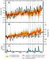
Fig. 1.

Modeled and observed SST changes in tropical cyclogenesis regions and observed changes in stratospheric aerosol optical depth (SAOD). Time series of monthly mean, spatially averaged SST anomalies are for the ACR (A) and PCR (B). Observational results are from the NOAA ERSST data set (16). Results for a second observational data set (17) are very similar (see Fig. 6). Model data from simulations of 20CEN climate change are partitioned into two groups, with and without volcanic forcing (V and No-V). All model data were low-pass filtered (with window width W = 21 months; see Fig. 7, which is published as supporting information on the PNAS web site) before formation of V and No-V averages (19). ERSST data were smoothed with the same filter. The yellow and gray envelopes are the 1σ and 2σ confidence intervals for the V averages, calculated with the smoothed data at each time t. Because most 20CEN experiments end in December 1999, V and No-V averages are calculated only until that month. ERSST data are shown through December 2005. All SST anomalies were defined relative to climatological monthly means over 1900 through 1909. This reference period was chosen for visual display purposes only, and it has no impact on subsequent trend analyses or variability estimates. The amplitudes of the observed and simulated SST variability are not directly comparable, because the latter was damped by averaging over different realizations and models. (C) Estimate of the SAOD (21). Dotted vertical lines denote the times of maximum SAOD during major volcanic eruptions.

Fig. 2.

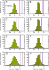
Comparison between observed and simulated SST changes in the ACR (A, C, E, and G) and PCR (B, D, F, and H). Results are expressed as the total linear change, b × n, where b is the slope parameter of the least-squares linear trend (in °C/month) and n is the total number of months. Trend comparisons are made on four different timescales: 100 years (A and B), 50 years (C and D), 30 years (E and F), and 20 years (G and H). Observed ACR and PCR SST trends from HadISST and ERSST were calculated over the periods 1906–2005, 1956–2005, 1976–2005, and 1986–2005. Sampling distributions of unforced SST trends on 100-, 50-, 30-, and 20-year timescales were computed as described in the main text. For visual display purposes, unforced SST trends were fitted to segments of the ACR and PCR anomaly time series that overlapped by all but 10 years. For the century-timescale results, this procedure yields 698 unforced SST trends for each tropical cyclogenesis region. Unforced trends are plotted in the form of histograms. Very similar (but less smooth) histograms are obtained if trends are fitted to nonoverlapping segments of control run SST data. Red and blue vertical lines indicate observed SST trends in the HadISST and ERSST data, respectively.

Fig. 3.

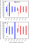
Estimates of the percentage contribution of external forcing to observed SST changes in the ACR (A) and PCR (B). Results are for F₁ (solid bars) and F₂ (circles and thin error bars). For definitions of F₁ and F₂, refer to main text. In computing F₁, model estimates of s_CTL were obtained from histograms similar to those shown in Fig. 2, but based on trends fitted to nonoverlapping rather than overlapping segments of SST time series.

Fig. 4.

Comparison of basic statistical properties of simulated and observed SSTs in the ACR and PCR. Results are for climatological annual means (A), temporal standard deviations of unfiltered (B) and filtered (C) anomaly data, and least-squares linear trends over 1900–1999 (D). For each statistic, ACR and PCR results are displayed in the form of scatter plots. Model results are individual 20CEN realizations and are partitioned into V and No-V models (colored circles and triangles, respectively). Observations are from ERSST and HadISST. All calculations involve monthly mean, spatially averaged anomaly data for the period January 1900 through December 1999. For anomaly definition and sources of data, refer to Fig. 1. The dashed horizontal and vertical lines in A–C are at the locations of the ERSST and HadISST values, and they facilitate visual comparison of the modeled and observed results. The black crosses centered on the observed trends in D are the 2σ trend confidence intervals, adjusted for temporal autocorrelation effects (see Supporting Text). The dashed lines in D denote the upper and lower limits of these confidence intervals.

Fig. 5.

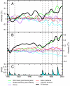
Contribution of different external forcings to SST changes in tropical cyclogenesis regions. (A and B) Results are for the ACR (A) and PCR (B) and are from a 20CEN run and single-forcing experiments performed with the PCM (27). Each result is the low-pass filtered average of a four-member ensemble, with window width W = 145 months. For anomaly definition, refer to Fig. 1. Stratospheric aerosol optical depth (21) is also shown (C).

References

1. Gray WM. Mon Weather Rev. 1968;96:669–700.
1. Emanuel KA. Nature. 1987;326:483–485.
1. Holland GJ. J Atmos Sci. 1997;54:2519–2541.
1. Raper SCB. In: Climate and Sea Level Change: Observations, Projections and Implications. Warrick RA, Barrow EM, Wigley TML, editors. Cambridge, UK: Cambridge Univ Press; 1993. pp. 192–212.
1. Knutson TR, Tuleya RE. J Clim. 2004;17:3477–3493.
Publication types