Neural mechanism for stochastic behaviour during a competitive game

Abstract

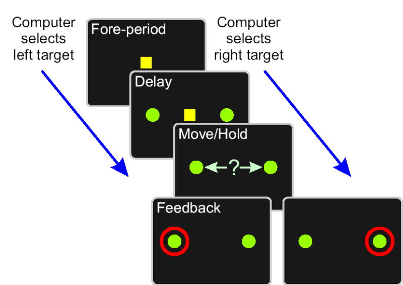
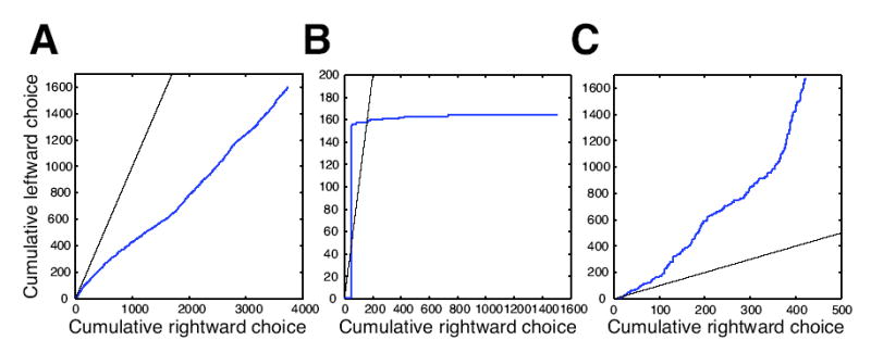
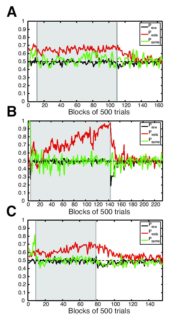
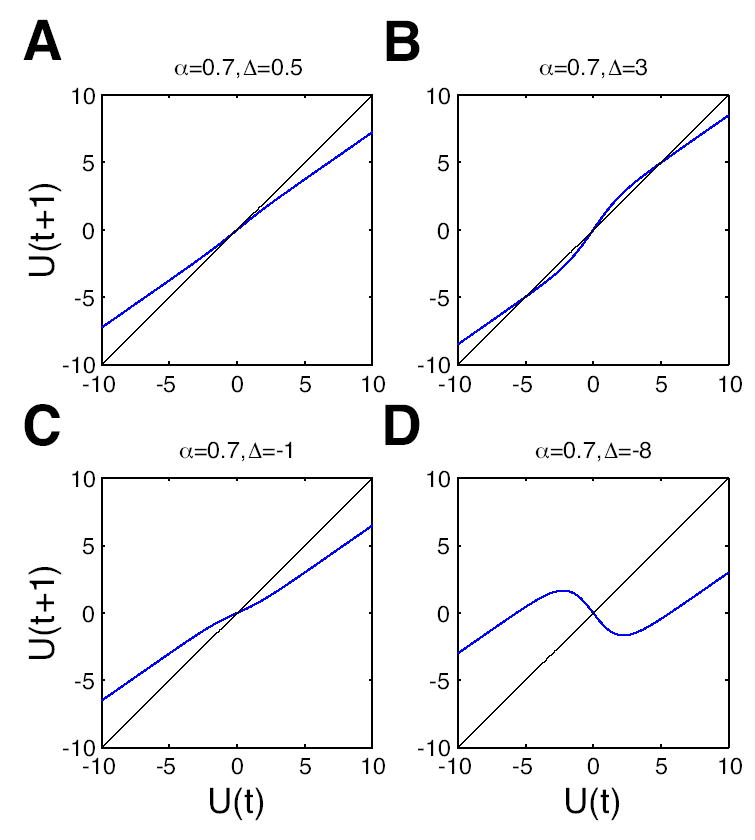
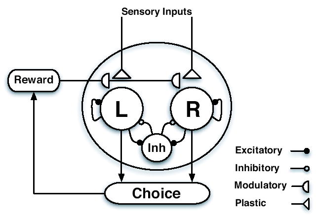
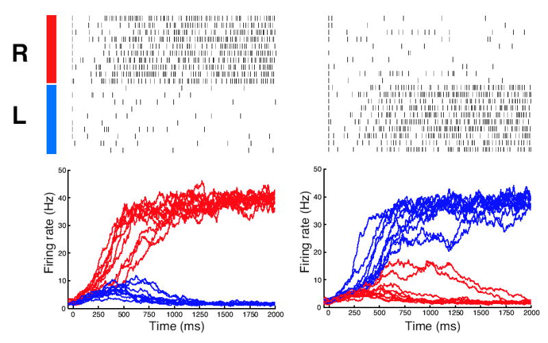
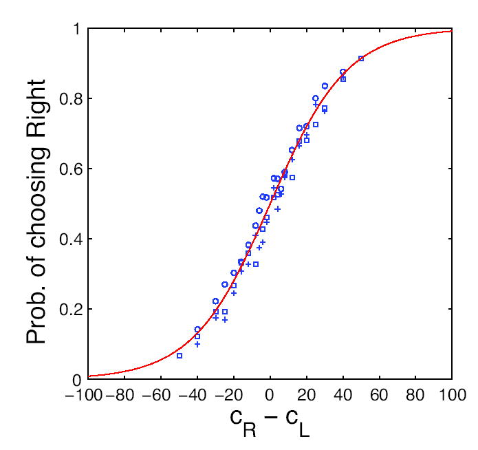
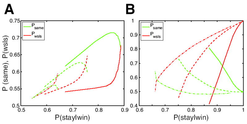
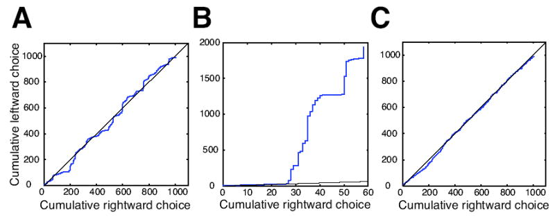
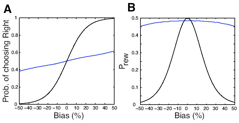
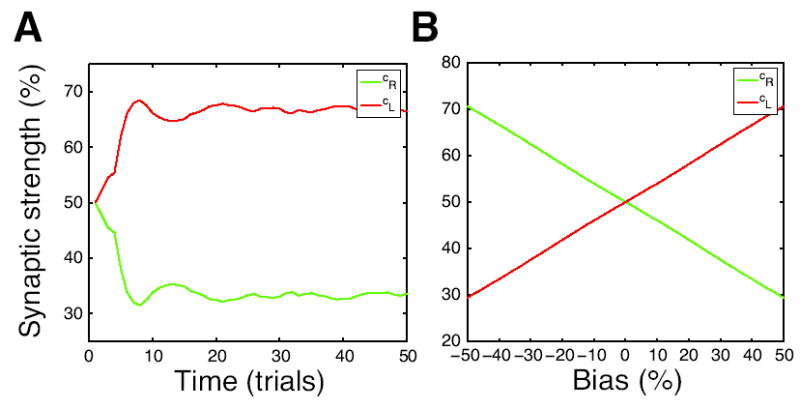
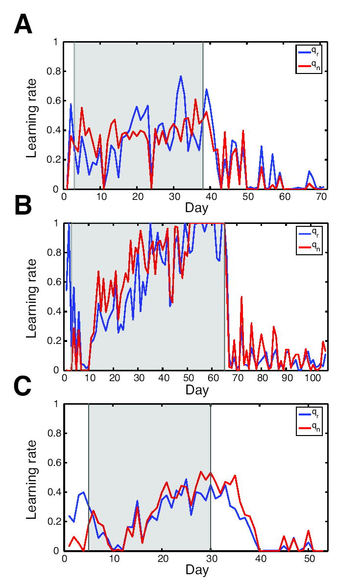
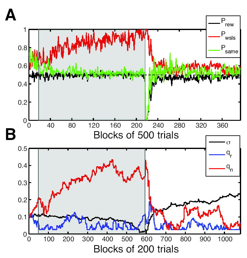
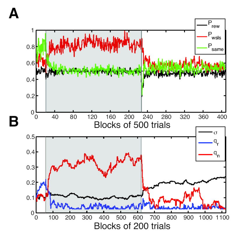
Previous studies have shown that non-human primates can generate highly stochastic choice behaviour, especially when this is required during a competitive interaction with another agent. To understand the neural mechanism of such dynamic choice behaviour, we propose a biologically plausible model of decision making endowed with synaptic plasticity that follows a reward-dependent stochastic Hebbian learning rule. This model constitutes a biophysical implementation of reinforcement learning, and it reproduces salient features of behavioural data from an experiment with monkeys playing a matching pennies game. Due to interaction with an opponent and learning dynamics, the model generates quasi-random behaviour robustly in spite of intrinsic biases. Furthermore, non-random choice behaviour can also emerge when the model plays against a non-interactive opponent, as observed in the monkey experiment. Finally, when combined with a meta-learning algorithm, our model accounts for the slow drift in the animal's strategy based on a process of reward maximization.

Figure 1

Spatial layout and temporal sequence of the free-choice task.

Figure 2

Instability in monkeys’ choice behavior in algorithm 0. The cumulative choices of the leftward target is plotted against the cumulative choices of the rightward target in three different monkeys (in the last 2 days of algorithm 0). (A) Choice behavior in monkey C was the most stable but it was biased toward the rightward target. (B) Monkey E showed very unstable choice behavior, such that at the end it chose only the rightward target. (C) In monkey F, the choice behavior was biased toward the leftward target. There are switches between the two targets but lengths of consecutive choices on the leftward target are larger. The black line corresponds to the choices made with equal probabilities.

Figure 3

Slow change in monkeys’ choice behavior over the course of the experiment. In each panel the average probability of choosing the same target as in the previous trial, P_same, probability of using WSLS strategy, P_wsls, and probability of harvesting reward, P_rew, are plotted for each monkey; (A): monkey C, (B) monkey E, (C) monkey F. The gradual change in P_wsls is present in all monkeys’ choice behavior but it is most prominent in the behavior of monkey E. Each probability is computed over a block of 500 trials. To distinguish the behavior in three different algorithms, blocks in algorithm 1 are shaded.

Figure 4

Stability analysis of the reinforcement learning model in algorithm 0. A steady state is given by the intersection of the update rule (blue curve) and the identity line (block line). For a fixed value of α, as the absolute value of Δ becomes larger, choice behavior at P_R = 0.5, or equivalently at U(t) = 0, becomes unstable. As shown in the top panels, if Δ is positive, as Δ increases the stable steady-state at U(t) = 0 (A) becomes unstable and two new stable steady-states emerge (B). Bottom panels (C and D) show the case in which Δ is negative. In this case a more negative value of Δ results in instability at U(t) = 0 (D). This instability results in alternation between the two targets.

Figure 5

Schematic model architecture. The core of the model consists of two populations of excitatory neurons which are selective to the two target stimuli and compete against each other through feedback inhibition. Upon the presentation of stimuli, neurons in the two selective populations receive similar inputs through plastic synapses. At the end of each trial these plastic synapses undergo a stochastic Hebbian learning rule which is gated by the all-or-none reward signal.

Figure 6

Examples of neural activity in the decision-making network in 20 simulated trials. The left panels show the population activity of the neurons, and the spike trains of example neurons in the two selective populations in trials in which the right population (red traces) wins the competition. Similarly the right panels show the activity in trials in which the left population (blue traces) wins the competition. In these simulations the synaptic strength onto the right populations is set to c_R = 52%, and synaptic strength onto the left populations is set to c_L = 48%.

Figure 7

Choice behavior of the decision-making network as a function of the difference in synaptic strengths. The choice probability is extracted from the full network simulations (400 trials for each set of synaptic strengths). Different symbols represent different sets of synaptic strength with different overall synaptic strength c_R + c_L = 60% (plus), 100% (square), 140% (circle). The red curve shows a sigmoid function (Eq. 6, σ=21%) fit to all data points.

Figure 8

Performance of the model with different learning rules in algorithm 1. (A) In the model with choice-specific learning rule, the probability of choosing the same target in two consecutive trials, P_same, mostly increases as the probability of WSLS strategy, P_wsls, increases. In addition there is a limit for P_wsls in this model. (B) In the model with belief-dependent learning rule, P_same decreases as the P_wsls increase, and P_wsls can reach to value close to 1. If σ value is large, P_wsls can vary over a large range while P_same is close to 0.5, consistent with the monkeys’ choice behavior. For these simulations the q₊ (or q_r) is fixed at 0.1 while q₋ (or q_n) is varied in the range of [0.025,0.825]. The value of σ. is set to 5%(solid), 10% (dash), and 20% (dot-dash).

Figure 9

Examples of different model’s choice behavior in algorithm 0. The model shows different choice behaviors depending on the learning parameters (for fixed σ = 10%). (A) For model parameters of q_r = 0.035, q_n = 0.03, the condition for a stable steady-state at P_R = 0.5 is met so the two targets are chosen with equal probability. (B) For q_r = 0.09, q_n = 0.03 the stable steady-state at P_R = 0.5 is not fulfilled and two new stable steady-states emerge. As a result, the model randomly shows a strong bias for one of the choices (in this example for the leftward choice). (C) If q_r = 0.1, q_n = 0.7 the only steady state at P_R = 0.5 is unstable and the model mostly alternates between the two choices. The black line shows the unity line.

Figure 10

Choice probability and performance of the model with an intrinsic bias. (A) The black curve shows the probability of choosing the rightward target for a given intrinsic bias, when the plastic synapses are not updated (or there is no feedback). The blue curve shows the probability of choosing the rightward target for the same model which plays against the computer in algorithm 1 and plastic synapses are updated. The bias in the model is drastically reduced, due to feedback and learning dynamics. (B) Performance of the model with an intrinsic bias. The probability of obtaining reward is plotted for different intrinsic biases while the model plays against the computer opponent in algorithm 1 (blue curve). The black curve shows the harvesting rate if the synapses are not updated and only the intrinsic bias determines the choice probability. For each value of the bias (from −50 to 50 with intervals of 1) the average in each condition is computed over 400 days (each day consists of 1000 ± 200 trials) of the experiment and the model parameters are set to q_r = 0.1, q_n = 0.2, and σ = 10%.

Figure 11

Intrinsic bias can be compensated by plastic synapses. (A) Time course of the average synaptic strengths, c_R and c_L, in algorithm 1. Within about 10 trials the difference between the two synaptic strengths increases to compensate for the intrinsic bias. In this simulation the rightward choice receives an additional constant input which is equivalent to 40% difference in synaptic strengths. The average is computed over 1000 sessions. (B) The average synaptic strengths for different values of intrinsic bias. As the intrinsic bias increases the difference in synaptic strengths also increases. The averages are computed over 1000 sessions for each intrinsic bias. The model parameters are set to q_r = 0.1, q_n = 0.2, and σ = 10%.

Figure 12

Maximum likelihood estimate of the model parameters. These parameters are obtained from fitting the choice behavior of three monkeys in each day of the experiment; (A) monkey C, (B) monkey E, (C) monkey F. The gradual change in the learning parameters during the experiment is another indication that monkeys changed their strategies continuously. Consistent with the results obtained in Sec. 5.1, in algorithm 0 q_r > q_n which explains the observed unstable choice behavior around P_R = 0.5. During algorithm 1, in all monkeys both learning rates increase which result in increase in the use of WSLS strategy. During algorithm 2 the learning rates decrease which shows that the only possible way to play randomly is to have slow learning. For these fittings, the value of σ is fixed at 50%.

Figure 13

An example of the model’s average choice behavior in 200 days of the experiment. When the meta-learning is active the model’s choice behavior is adjusted according to the algorithm used by the computer opponent. (A) Time courses of different measures of the model’s choice behavior (average over blocks of 500 trials). Blocks during algorithm 1 are shaded. (B) The model parameters are adjusted in each 200 trials according to meta-learning algorithm. The initial values for the model parameters are q_r = q_n = 0.1 and σ = 10% and meta-learning parameters used for updating the learning rates (q_r and q_n) are ν_q = 2, and ε_q = 0.002, and for updating the noise level σ, ν_s = 5, ε_s = 0.005. The time constants for averaging reward are set to τ₁ = 100 and τ₂ = 400 trials.

Figure 14

Another example of the model’s average choice behavior in 200 days of the experiment. The model parameters are similar to those used in Fig. 13.

References

1. Amit DJ, Fusi S. Dynamic learning in neural networks with material synapses. Neural Computation. 1994;6:957–982.
1. Bar-Hillel M, Wagenaar WA. The perception of randomness. Advances in Applied Mathematics. 1991;12:428–454.
1. Barraclough DJ, Conroy ML, Lee D. Prefrontal cortex and decision making in a mixed-strategy game. Nature Neuroscience. 2004;7:404–410. - PubMed
1. Berns GS, Sejnowski TJ. A computational model of how the basal ganglia produce sequences. Journal of Cognitive Neuroscience. 1998;10:108–121. - PubMed
1. Brunel N, Wang XJ. Effects of neuromodulation in a cortical network model of object working memory dominated by recurrent inhibition. Journal of Computational Neuroscience. 2001;11:63–85. - PubMed
Publication types
LinkOut - more resources