Biological systems modeling and analysis: a biomolecular technique of the twenty-first century

Abstract

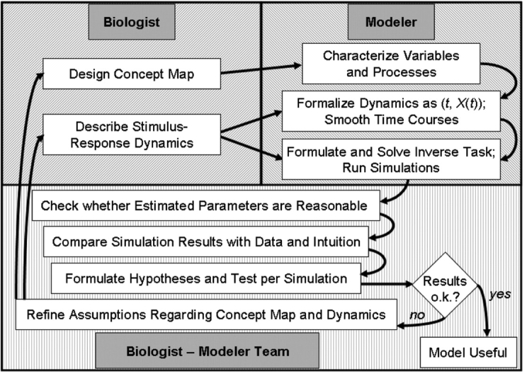
It is proposed that computational systems biology should be considered a biomolecular technique of the twenty-first century, because it complements experimental biology and bioinformatics in unique ways that will eventually lead to insights and a depth of understanding not achievable without systems approaches. This article begins with a summary of traditional and novel modeling techniques. In the second part, it proposes concept map modeling as a useful link between experimental biology and biological systems modeling and analysis. Concept map modeling requires the collaboration between biologist and modeler. The biologist designs a regulated connectivity diagram of processes comprising a biological system and also provides semi-quantitative information on stimuli and measured or expected responses of the system. The modeler converts this information through methods of forward and inverse modeling into a mathematical construct that can be used for simulations and to generate and test new hypotheses. The biologist and the modeler collaboratively interpret the results and devise improved concept maps. The third part of the article describes software, BST-Box, supporting the various modeling activities.

FIGURE 1

Concept map summarizing siRNA knockdown studies demonstrating how effects of the physico-mechanical environment are mediated by integrins. (Barbara Boyan, personal commumication; scientific details can be found in reference .)

FIGURE 2

Flow diagram of the proposed approach to formalizing biological concept maps.

FIGURE 3

Opening GUI of BSTBox as it is invoked in MATLAB using the command “BST”; the user may opt to create a new map or to retrieve an earlier created and stored map from a MATLAB data file.

FIGURE 4

Simplified representation of glycolysis and lactate production in L. lactis. Black arrows show flow of material, while grey arrows indicate signals; subscripted Xs designate dependent variables in the model equations. Metabolites without symbolic names were used as offline variables (see text); pyruvate is shown only for completeness but is not explicitly modeled. Abbreviations: G6P = glucose 6-phosphate; FBP = fructose 1,6-bisphosphate; 3-PGA = 3-phosphoglycerate; PEP = phosphoenolpyruvate; ATP = adenosine tri-phosphate; ADP = adenosine diphosphate; p_i = inorganic phosphate

FIGURE 5

Different functionalities of BSTBox are embedded in separate tabs, which unlock progressively as the user transitions from one stage of the modeling process to the next. When creating a new biochemical map, the first tab, “Select Data Set,” allows the user to specify which MS-Excel sheet contains the raw and smoothed data, and also which columns contain the time data and the experimental measurements of the metabolite levels. At this step, the distinction is made between metabolites to be modeled and metabolites to be treated as offline. Upon specification, the user clicks “Done” to proceed to the next tab.

FIGURE 6

The second tab, “Specify Map Configuration,” allows the user to enumerate all processes that determine the dynamics of each metabolite. The user specifies the numbers of influxes and effluxes that determine the concentrations of each metabolite, and for each of these processes lists the variables that directly influence that process. In effect, the user provides a tabular description of what would otherwise be a graphical biochemical map. The user may also add constraints, such as the conservation of mass between precursors and products. The corresponding Gui for this task is invoked by clicking the button “Add Constraints” (see Figure 7). When done, the user proceeds to the next tab to generate and view the functional form of the model equations.

FIGURE 7

This GUI permits specification of precursor-product relationships between different influx and efflux terms. For each metabolite, the user may browse the list of processes (influxes and effluxes) that determine the levels of that metabolite. Given an unbranched pathway, such as in the case of Lactococcus, the user may constrain the efflux from one pool to be equal to the influx into another pool. Currently, BSTBox supports only one-to-one constraint specifications.

FIGURE 8

The tab “View Functional Model” allows the user to generate the necessary system of BST equations by the simple click of a button. Due to the rigorous rules of BST, BSTBox has enough information in the lists of processes and components to generate a (not yet parameterized) model and to present the model equations in a variety of formats. When done, the user proceeds to the next tab to specify or edit the time-course data interactively for all metabolites involved.

FIGURE 9

The tab “Edit Time Series Data” allows the user to view the raw experimental time-course data and to smooth them; it is easy to toggle between the raw or smooth data sets by means of a drop-down menu. The user may select multiple metabolites to view their time courses simultaneously. When editing these time plots, BSTBox invokes MATLAB’s spline Toolbox, shown in Figure 10, to allow the user to edit and approximate these time curves using cubic splines. In the absence of experimental observations, users of BSTBox have the ability to start with time courses (in MS-Excel) that had not been measured but are expected based on the biologist’s experience and intuition, load these data into BSTBox, smooth them, specify a model, and test hypotheses with this model. The user has the option to export the edited time-series data as an MS-Excel file. As a future enhancement, the user will be allowed to import and update these data sets with additional experimental observations. When done, the user proceeds to the next tab to estimate or specify values for the system parameters.

FIGURE 10

splineTool for editing time-series data. BSTBox provides access to this MATLAB tool such that the user’s time-series data are directly loaded into the Spline Tool interface and made available for editing purposes. The user may add or delete time points using the right click menu in the upper plot area; the lower plot shows the error in the approximated curve from the original (raw) time-series data; the GUI elements on the left hand allow the user to choose between multiple approximation schemes such a cubic spline interpolation or least-squares approximation; on the lower left-hand side, the user may manually edit each data point in the table of values listed here. All changes are preserved and saved in BSTBox.

FIGURE 11

Smoothed time-course data; each of these curves was manually enhanced, using the spline Tool interface. A cubic spline interpolation was used and data points were manually deleted from the set of points available, generating the curves shown here. Magenta: raw data; blue: manually smoothed data

FIGURE 12

General architecture of an optimization scheme for parameter estimation. Three sets of “inputs” are the measured or hypothetical data, the symbolic (not yet parameterized) model equations, and initial guesses for all parameter values. The optimization algorithm begins by solving the equations with the guessed parameter values and computing the residual error between the solution and the data. It then determines new parameter guesses, solves again, and computes the error again. This cycle is iterated thousands of times, in an attempt to minimize the error between the computed model time courses and the data curves (“shrinking” of the green arrows, indicating that the residual error is to be minimized).

FIGURE 13

The “Estimate Parameters” tab provides an interface to call various parameter estimation techniques. From the radio button selection in the top panel, a user can select either slope-based and/or ODE-based local optimization, or a global optimization technique such as a genetic algorithm. The user may change the default settings for the bounds of parameter search, initial parameter guess, and acceptable residual error. When using ODE-based estimation, the user may also specify the desired numerical solver to be employed for integrating the equations. The user furthermore chooses whether to search for parameters that would make the underlying model fit the raw data or the smoothed data and determines the time period of the data over which the parameters should be optimized. Building upon the offline-spline-based approximation framework, the user can estimate parameters for either the entire system simultaneously, for one parameter at a time, or for combination(s) thereof. Finally, the user has the option to bypass parameter estimation if the parameters are already available. The user can directly type these parameter values into the GUI and proceed to the next tab to simulate the system. In such a scenario, the user does not have to provide time-series data, and only initial values at the start time are expected in the MS-Excel file.

FIGURE 14

model fits (lines) to the Lactococcus data (symbols) of our case study, obtained with parameters estimated using regular ODE-based optimization scheme. The initial parameter guesses were set to +0.5 or to −0.5, depending on the sign of each parameter, which is usually known from the tenets of BST. The lsqcurvefit routine, available within the MATLAB Optimization Toolbox, was used. The complete optimization took about 20 min.

FIGURE 15

The tab “Run Simulation” uses the functional model, combined with initial time values and final parameter values from previous tabs to simulate the system. The user may choose to simulate either the entire system, one component at a time, or a subset of components. As earlier, spline approximations are used for all offline components. For assessments of quality, The GUI displays the results together with the data or in separate windows. It is easy with this interface to conduct perturbation studies, by changing the initial values for one or some of the metabolites. The user can also choose different integration schemes to simulate the system. Upon the successful execution of the simulation, the user may export the simulation results, which include all categories of time-series data—raw, smoothed/edited and simulated—to an MS-Excel file.

References

1. Voit EO. Models-of-data and models-of processes in the post-genomic era. Special Issue in honor of John A. Jacquez. Math Biosci 2002;180:263–274. - PubMed
1. Leicester HM. Development of Biochemical Concepts from Ancient to Modern Times. 1974, Cambridge, MA: Harvard University Press.
1. Voit EO, Schwacke JH. Understanding through Modeling, in Konopka AK, Editor. Systems Biolog y: Principles, Methods, and Concepts, in press, 2006.
1. Crampin EJ, Halstead M, Hunter P, Nielsen P, Noble D, Smith N, et al. Computational physiology and the Physiome Project. Exp Physiol 2004;89:1–26. - PubMed
1. Westerhoff HV, Palsson BO. The evolution of molecular biology into systems biology. Nat Biotechnol 2004;22:1249–52. - PubMed
Publication types
LinkOut - more resources