Dynamic spatial processing originates in early visual pathways

Abstract

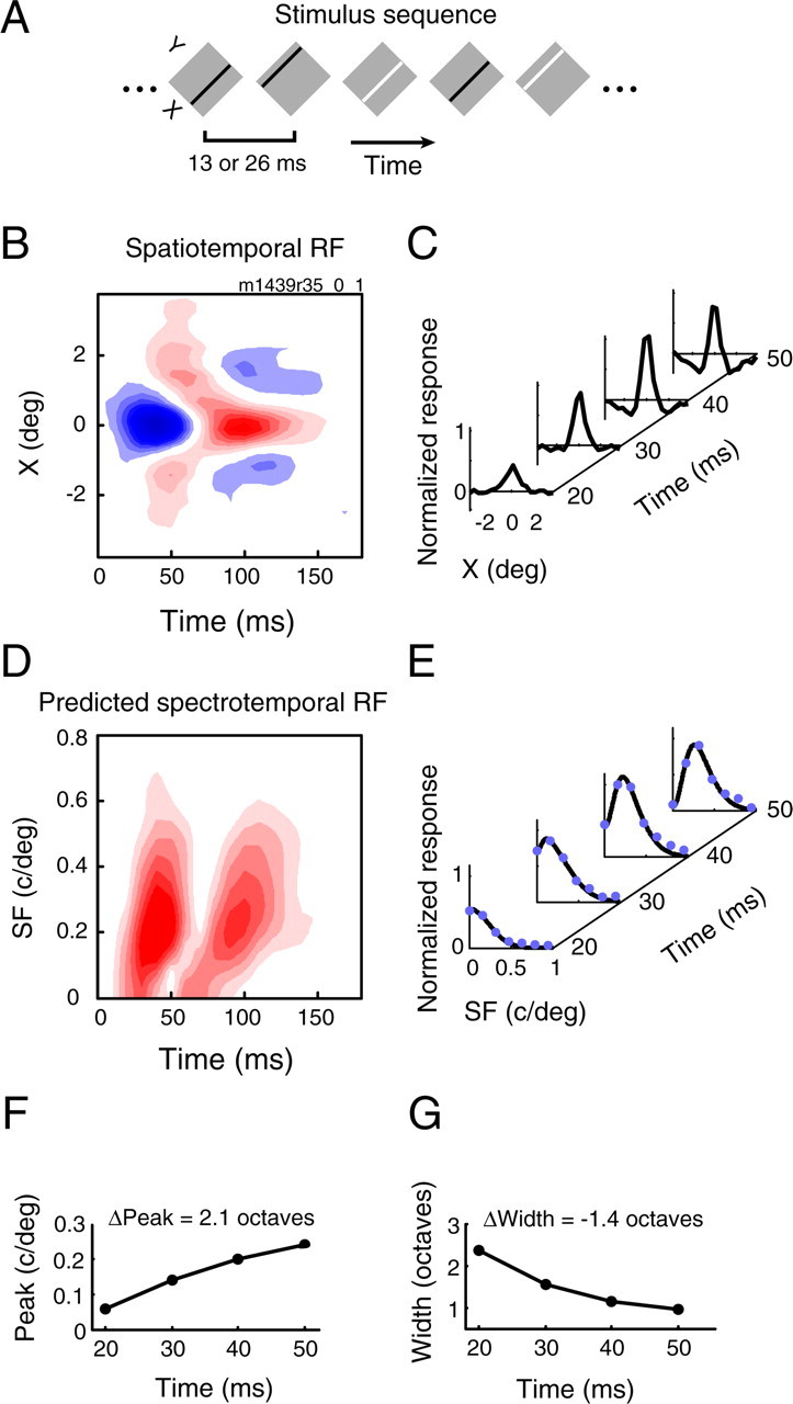
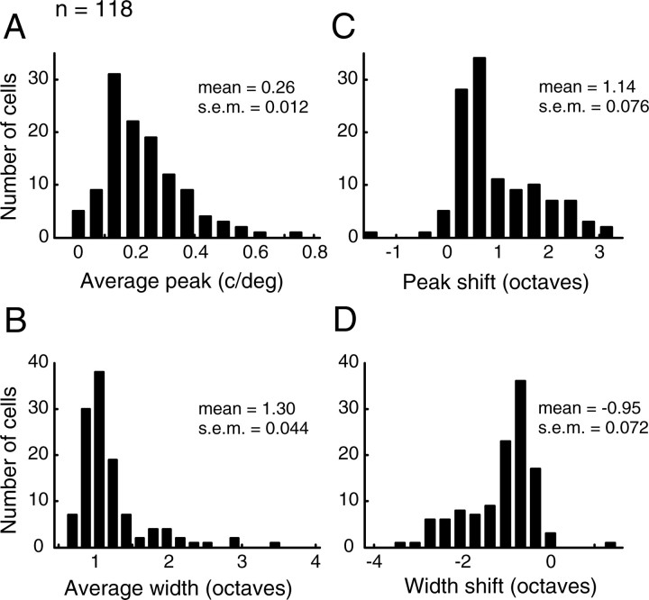
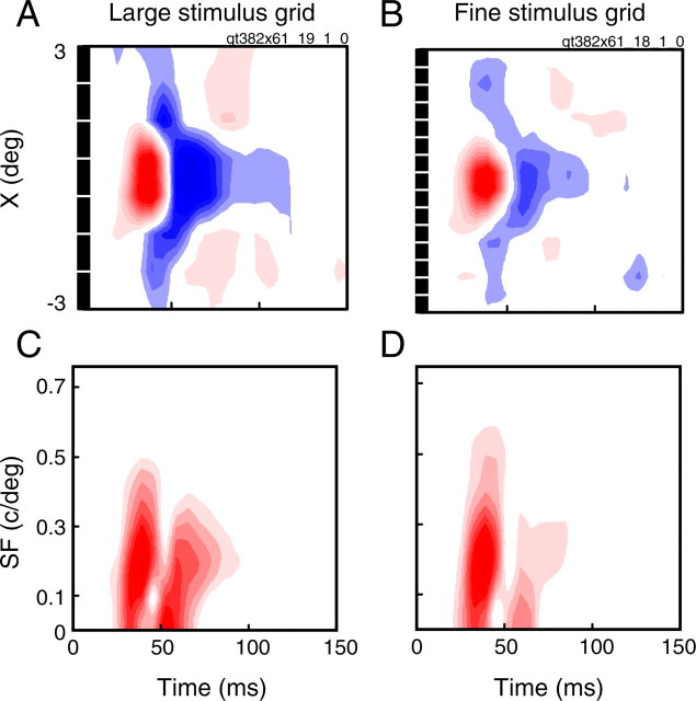
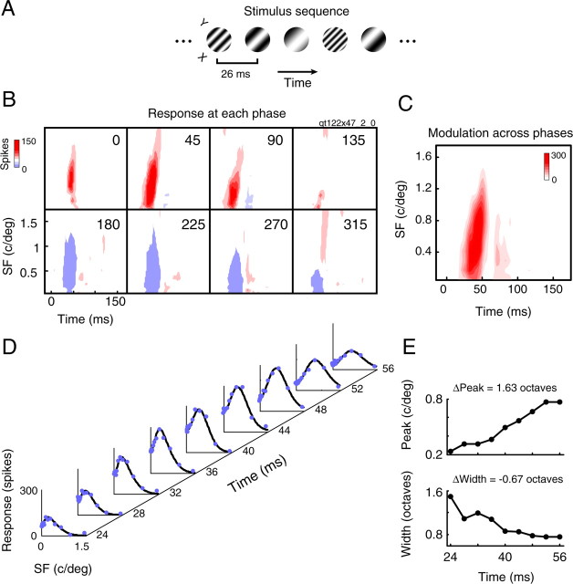
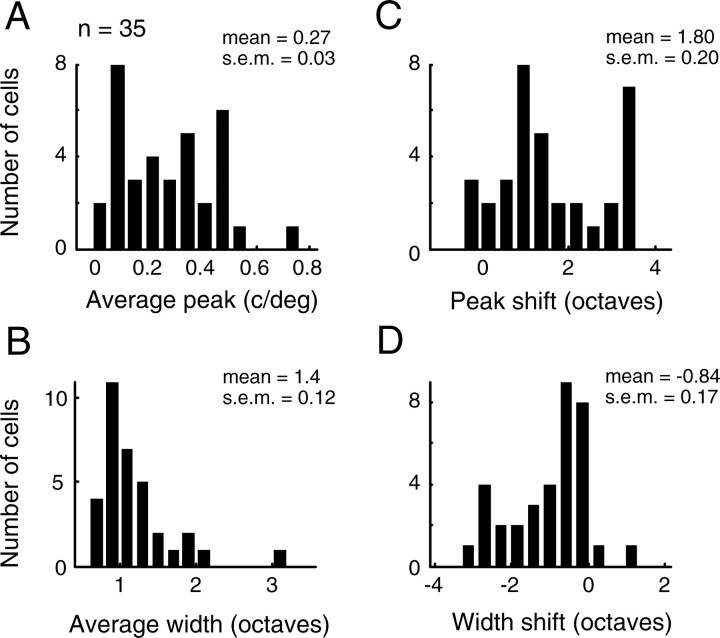
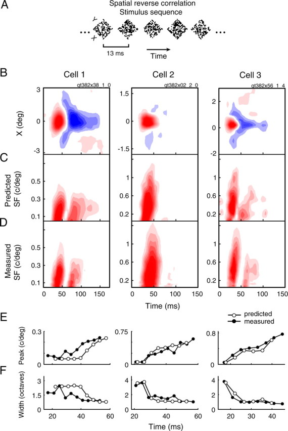
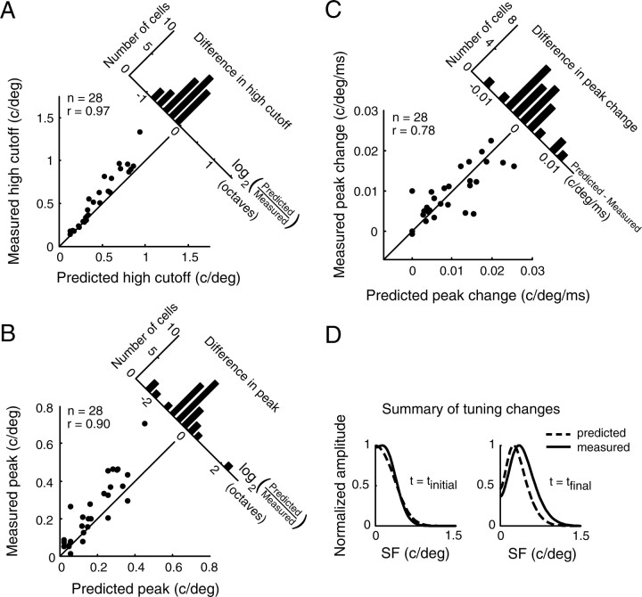
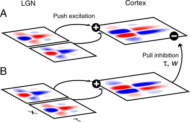
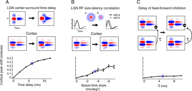
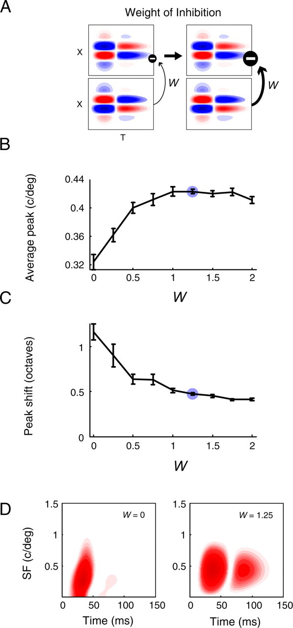
A variety of studies in the visual system demonstrate that coarse spatial features are processed before those of fine detail. This aspect of visual processing is assumed to originate in striate cortex, where single cells exhibit a refinement of spatial frequency tuning over the duration of their response. However, in early visual pathways, well known temporal differences are present between center and surround components of receptive fields. Specifically, response latency of the receptive field center is relatively shorter than that of the surround. This spatiotemporal inseparability could provide the basis of coarse-to-fine dynamics in early and subsequent visual areas. We have investigated this possibility with three separate approaches. First, we predict spatial-frequency tuning dynamics from the spatiotemporal receptive fields of 118 cells in the lateral geniculate nucleus (LGN). Second, we compare these linear predictions to measurements of tuning dynamics obtained with a subspace reverse correlation technique. We find that tuning evolves dramatically in thalamic cells, and that tuning changes are generally consistent with the temporal differences between spatiotemporal receptive field components. Third, we use a model to examine how different sources of dynamic input from early visual pathways can affect tuning in cortical cells. We identify two mechanisms capable of producing substantial dynamics at the cortical level: (1) the center-surround delay in individual LGN neurons, and (2) convergent input from multiple cells with different receptive field sizes and response latencies. Overall, our simulations suggest that coarse-to-fine tuning in the visual cortex can be generated completely by a feedforward process.

Figure 1.

Prediction of SF tuning dynamics from spatiotemporal RFs. A, The stimulus sequence used to map spatiotemporal RFs was one-dimensional sparse noise. Elongated dark and light bars, aligned to a cell's preferred orientation, were randomly displayed at 20 or 30 positions over the RF. B, The spatiotemporal RF of an OFF-center cell. RFs are plotted as contour maps, where blue and red contours enclose dark and bright excitatory regions, respectively. For this and all other contour maps, each contour indicates a 10% decrement from the maximum amplitude. C, Time slices from 20 to 50 ms show the evolution of the spatial response over time, and in particular, the delayed development of the surround. D, Fourier analysis of the spatiotemporal RF yields the linear prediction of the spectrotemporal RF. E, Rightward tilted contours in the SF–time plane indicate coarse-to-fine dynamics, and time slices show a clear change from low to bandpass SF tuning. Solid blue dots mark data points whereas black curves show the DOG least-squares fit used to obtain tuning parameters for each time point. F, G, Graphs of tuning parameters over time. The peak SF (F) increases, and the half-width (G) decreases. Half- width is defined as follows: bw = log₂(SF_high/SF_peak), where SF_peak is the optimal SF and SF_high is the SF to the right of SF_peak at which amplitude falls to half the maximum value.

Figure 2.

Population distributions of predicted tuning parameters and parameter changes over time. A, B, Histograms of the peak SF (A) and half-width (B) for our sample of LGN neurons (n = 118). Average tuning parameters describe the tuning curve obtained by integrating the spectrotemporal map from t_initial to t_final (∼30 ms). C, D, Distributions of changes in peak SF and tuning width. Peak shift is defined as log₂[SF_peak(t_final)/SF_peak(t_initial)], and the shift in width is bw(t_final) − bw(t_initial). Both the mean of the peak shift (1.14 ± 0.076 octaves, mean ± SEM) and the mean of the width shift (−0.95 ± 0.072 octaves, mean ± SEM) were significantly different from zero (p ≈ 0 and p ≈ 0, two-tailed t test).

Figure 3.

Spatiotemporal RFs of a single neuron obtained with different stimulus grid sizes. A, C, The mapped spatiotemporal RF (A) and predicted spectrotemporal RF (C) obtained with an 8 × 8 stimulus grid. B, D, The mapped spatiotemporal RF (B) and predicted spectrotemporal RF (D) obtained with a 16 × 16 stimulus grid. Black boxes along the X dimension of the spatiotemporal RFs show the positions and sizes of each stimulus pixel. The stimuli used in A are too large to capture the full narrowing of the center component which is seen in B. This corresponds to a reduction in the high SF cutoff in the SF domain (compare C, D). However, the large stimuli are much more effective in eliciting a response from the surround.

Figure 4.

SF tuning dynamics measured with subspace reverse correlation. A, The stimulus for reverse correlation in the SF domain was a randomized sequence of iso-oriented sinusoidal gratings, each with one of 15 possible SFs and eight possible phases. Gratings were presented consecutively every two video frames (26 ms). B, Spectrotemporal RFs computed at each phase after 200 repetitions of the stimulus. Red and blue contours correspond to responses above and below the baseline level, respectively. C, Because responses are strongly linear with respect to phase, we compute the modulation over phase at each SF and correlation delay for further analysis. D, Time slices approximately spanning the first phase of the response reveal prominent changes in SF tuning. DOG fits (black curves) to the raw data (solid blue dots) were used to estimate tuning parameters. E, Both the peak SF (top) and the half-width (bottom) change over time in a coarse-to-fine manner.

Figure 5.

Population distributions of measured tuning parameters and parameter changes over time. A, B, Histograms of the peak SF (A) and half-width (B) obtained with subspace reverse correlation for a sample of 35 LGN neurons. C, D, The distributions of changes in peak SF and tuning width. Both the mean of the peak shift (1.8 ± 0.20 octaves, mean ± SEM) and the mean of the width shift (−0.84 ± 0.17 octaves, mean ± SEM) are significantly different from zero (p < 10⁻⁹ and p < 0.0001, respectively, two-tailed t test).

Figure 6.

Predicted and measured SF tuning for three example cells. A, For comparing predicted and measured SF tuning, we used a slightly different version of spatial reverse correlation. Here, the stimulus sequence was 2D dense noise, where each frame displayed a 16 × 16 or 32 × 32 grid of black and white squares. B, Spatiotemporal RFs mapped with the sequence in A for three representative LGN cells. C, Predicted spectrotemporal RFs for each cell, obtained by taking the Fourier transform of their spatial maps. D, Measured spectrotemporal RFs, obtained with the stimulus depicted in Figure 3A. E, F, Temporal changes in the tuning peak (E) and half-width (F) are shown for both the predicted (open circles) and measured (filled circles) tuning curves.

Figure 7.

Population comparison of predicted and measured SF tuning. A, Scatter plot of predicted and measured high cutoff values for a sample of 28 neurons. There is a strong correlation (r = 0.97; p < 10⁻¹⁵, linear regression), although predictions clearly deviate from measurements. The differences between these values, computed as the log ratio of predicted SF_high to measured SF_high, are displayed in a histogram (top right). The mean difference is significantly different from zero (−0.22 ± 0.04 octaves, mean ± SEM; p < 10⁻⁵, two-tailed t test). B, Scatter plot of average predicted tuning peaks and measured tuning peaks. The data are highly correlated (r = 0.90; p < 10⁻⁹, linear regression) and most points lie above the y = x line, indicating a higher peak when SF tuning was measured directly. The mean difference, computed analogously to the difference in high cutoff, is significantly different from zero (−0.42 ± 0.16 octaves, mean ± SEM; p < 0.05, two-tailed t test). C, Scatter plot of the predicted changes and measured changes in tuning peak. The data are well correlated (r = 0.78; p < 10⁻⁶, linear regression) and points are roughly evenly distributed above and below the unity line. The differences between predicted and measured tuning changes are symmetrically distributed around zero. The mean of this distribution (3.6 × 10⁻⁴ ± 8.5 × 10⁻⁴ c/deg/ms, mean ± SEM) is not significantly different from zero (p > 0.5, two-tailed t test). D, A summary of SF tuning dynamics over the population of cells. Both predicted (dashed line) and measured (solid line) curves show a large shift from low-pass tuning at t_initial (left) to more bandpass tuning at t_final (right). However, for all time points, predicted tuning curves underestimate the true peak, as shown in B. Because this difference is roughly fixed over time, the predicted rate of peak change is relatively unaffected and correlates well to the measured value, as shown in C. Curves were generated by averaging the parameters of the best-fit DOG at the initial and final time point for each cell.

Figure 8.

A feedforward model examining mechanisms of SF dynamics in cortex. A, B, Responses of simple cells are modeled with a push–pull circuit. Excitatory input (A) to a cortical cell comes from spatially offset, although still overlapping, ON- and OFF-center LGN cells. The offset is exaggerated in this illustration for clarity. Inhibition (B) is provided by LGN cells with identical spatial position but opposite phase, after being routed through a cortical interneuron. The inhibition is parameterized with a time delay (τ) between excitation and inhibition, and a weight (W), which gives the relative level of inhibition compared with excitation.

Figure 9.

Effect of different model parameters on cortical tuning dynamics. A–C, Each diagram (top) illustrates the model parameter being explored and the effect on the cortical RF. Parameter values increase from left to right. Graphs (bottom) show the mean ± SEM shift in peak SF as a function of the model parameter, obtained after 15 simulations. Each set of simulations focused on a single variable; the other two parameters were fixed at zero and the inhibitory weight (W) was set to 1.25. Blue circles indicate average values found in previous studies (Ferster, 1988; Cai et al., 1997; Hirsch et al., 1998; Weng et al., 2005), which are also used in inhibitory weight simulations (Fig. 8). A, Cortical shift in peak SF as a function of the time delay between the center and surround in LGN RFs. B, Cortical shift in peak SF as a function of the slope relating response latency to RF size. A negative slope indicates that cells with larger RFs have shorter latencies than cells with smaller RFs. C, Cortical shift in peak SF as a function of the time delay (τ) between the arrival of excitation and inhibition in a cortical cell.

Figure 10.

Effect of inhibitory weight on cortical tuning dynamics. A–D, For simulations in which we vary the weight of inhibition (W), all other parameters are held fixed at the values marked by blue circles in Figure 9 (LGN center-surround delay, 6 ms; size-latency slope, −3.5 ms/deg²; inhibitory delay, 5 ms). The blue circles in B and C of this figure indicate the value of W used for simulations in Figure 9. A, A diagram depicting an increase (from left to right) in the weight of feedforward inhibition. B, The average peak SF increases as a function of W. C, The shift in peak SF decreases as inhibition increases, and plateaus at 0.4 octaves. D, Spectrotemporal RFs from the model elucidate the trends in B and C. Without inhibition (W = 0, left), cortical SF tuning mimics that of the LGN (compare with Fig. 4D): the initial response is low-pass, and over time the peak SF changes more than an octave. With relatively strong inhibition (W = 1.25, right), only stimuli that preferentially excite LGN cells of a single phase (i.e., stimuli with higher SFs) will produce a response in the cortical cell. Thus, the initial response is bandpass, and more moderate peak changes (∼0.4 octaves) occur as a result of input dynamics.

References

1. Albrecht DG. Visual cortex neurons in monkey and cat: effect of contrast on the spatial and temporal phase transfer functions. Vis Neurosci. 1995;12:1191–1210. - PubMed
1. Alonso JM, Usrey WM, Reid RC. Rules of connectivity between geniculate cells and simple cells in cat primary visual cortex. J Neurosci. 2001;21:4002–4015. - PMC - PubMed
1. Anzai A, Ohzawa I, Freeman RD. Neural mechanisms for encoding binocular disparity: receptive field position versus phase. J Neurophysiol. 1999;82:874–890. - PubMed
1. Bauman LA, Bonds AB. Inhibitory refinement of spatial frequency selectivity in single cells of the cat striate cortex. Vision Res. 1991;31:933–944. - PubMed
1. Bonin V, Mante V, Carandini M. The suppressive field of neurons in lateral geniculate nucleus. J Neurosci. 2005;25:10844–10856. - PMC - PubMed
Publication types
MeSH terms
LinkOut - more resources