Remapping in human visual cortex

Abstract

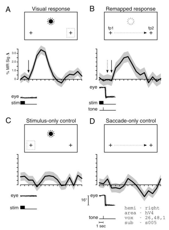
With each eye movement, stationary objects in the world change position on the retina, yet we perceive the world as stable. Spatial updating, or remapping, is one neural mechanism by which the brain compensates for shifts in the retinal image caused by voluntary eye movements. Remapping of a visual representation is believed to arise from a widespread neural circuit including parietal and frontal cortex. The current experiment tests the hypothesis that extrastriate visual areas in human cortex have access to remapped spatial information. We tested this hypothesis using functional magnetic resonance imaging (fMRI). We first identified the borders of several occipital lobe visual areas using standard retinotopic techniques. We then tested subjects while they performed a single-step saccade task analogous to the task used in neurophysiological studies in monkeys, and two conditions that control for visual and motor effects. We analyzed the fMRI time series data with a nonlinear, fully Bayesian hierarchical statistical model. We identified remapping as activity in the single-step task that could not be attributed to purely visual or oculomotor effects. The strength of remapping was roughly monotonic with position in the visual hierarchy: remapped responses were largest in areas V3A and hV4 and smallest in V1 and V2. These results demonstrate that updated visual representations are present in cortical areas that are directly linked to visual perception.

FIG. 1

Three task conditions. A: single-step task. Subject fixates a cross (FP1) located 8° to the left of screen center. After a variable period (1,000 · 200 ms), a salient stimulus appears in the right visual field and flickers on the screen for 1 s. The stimulus (full circles) activates contralateral (left) hemisphere visual cortex. Next, the stimulus is extinguished and a tone cues the subject to make a rightward eye movement to FP2. This saccade brings the screen location of the now-extinguished stimulus (empty circles) into the left visual field. After a variable period (2,000 · 200 ms), a 2nd tone instructs the subject to make a return saccade back to FP1. B: stimulus-only fixation task. Subject fixates FP1. After a variable period (1,000 · 200 ms), the visual stimulus appears in the periphery. The stimulus is extinguished after 1,000 ms. The trial ends after a variable fixation period (2,000 · 200 ms). C: saccade-only control task. Subject fixates FP1. After a variable period (2,000 · 200 ms), a tone cues the subject to make an eye movement to FP2. The subject fixates for a variable period (2,000 · 200 ms) until a 2nd tone cues them to make a return saccade. Dashed squares and arrows indicate the location of the eyes.

FIG. 2

Analysis of eye-position data. Eye traces from 64 trials of the single-step task (A), the saccade-only control task (B), and the stimulus-only control task (c). Calculated saccadic reaction time (SRT) is indicated by tick marks in A and B. This subject made 1 anticipatory saccade in the single-step task and 1 late saccade in the saccade-only task. Error trials were excluded from the analysis of fMRI data. D: no difference in saccade reaction time in trials of the single-step task (light gray bars) and saccade-only control task (dark gray bars). Saccadic reaction times across trials are represented using standard box-and-whisker plots (vertical lines at the center of each box indicate the median; box-ends indicate the quartiles).

FIG. 3

A: 16 slices were oriented perpendicular to the calcarine sulcus. Slices were 3 mm thick and covered the entire occipital lobe. B: 3-dimensional (3D) rendering of the cortical surface at the gray/white matter boundary. Shaded gray region indicates the cortical region of interest, shown as a flattened patch in the four panels below. Each disk in C-F shows the same flattened patch of cortex with a 50-mm radius. Gray background represents estimated cortical curvature: (dark gray, concave; light gray, convex). C: representation of polar angle. The stimulus was a rotating 15° checkerboard wedge. This map was used to define borders between the ventral portions of V1, V2, V3, and hV4. D: representation of visual eccentricity. The stimulus was an expanding/contracting 15° checkerboard annulus. In both C and D, hue represents the stimulus location that elicited the maximal response. E: response to contralateral visual stimulus in fixation task. F: response to the updated stimulus trace in the single-step task. In both E and F, hue (red-yellow) represents the magnitude of the response. Color opacity (transparent-opaque) represents the probability that the response to the stimulus was nonzero. Opacity values range from 0 to 1; the data are not thresholded.

FIG. 4

Hemodynamic responses in a single right hemisphere hV4 voxel that exhibits remapping. The cartoon in each panel shows the location of the stimuli on the screen. Horizontal eye position and timing of stimulus events are shown below (calibration bar, 16°). A: visual response in fixation task. A contralateral stimulus during fixation elicits a strong response. B: remapped response in single-step task. The subject fixates FP1 as a stimulus flickers in the ipsilateral visual field for 1 s. After 1 s, the stimulus is extinguished and a tone cues the subject to make a saccade to FP2. The saccade brings the screen location of the extinguished stimulus into the contralateral visual field. The remapped trace of the stimulus elicits a response. 1, onset time of the visual (- - -) and remapped response (—). C: stimulus-only control. Presentation of the stimulus in the ipsilateral visual field does not elicit a response in the absence of a saccade. D: saccade-only control. The saccade alone does not elicit a strong response in the absence of a stimulus. Each curve was estimated from responses on 64 trials. 1, 1 SE.

FIG. 5

Population activity in 3 task conditions. A: proportion of visually responsive voxels across all hemispheres in which responses reached a posterior probability threshold of q · 0.95. Light gray bars, responses to ipsilateral visual stimuli during stimulus-only fixation task (stim). Medium gray bars, responses to saccades in the absence of salient visual stimuli (sac). Dark gray bars, responses in the single-step task when a visual stimulus appears in the ipsilateral visual field and is followed by an ipsiversive saccade (sstep). The prevalence of voxels activated by the single-step task increases with position in the visual hierarchy. B: response magnitude in three conditions normalized by responses to contralateral visual stimuli. Magnitude estimates were averaged across all visually-responsive voxels within a region of interest (ROI) within a single hemisphere. Box-and-whisker plots indicate the distribution of response magnitudes across hemispheres. The strength of activity in the single-step task increases with position in the visual hierarchy.

FIG. 6

Responses in the single-step task are larger than responses in both control conditions. Each dot represents the average activity in all 3 conditions for a single hemisphere: ipsilateral responses in the single-step task, stimulus-only control condition, and saccade-only control condition were each averaged within hemisphere, normalized so that they sum to 1, and then plotted on triangular simplex plots. Position of a hemisphere in the simplex represents the selectivity of responses for each of the three conditions. Dotted horizontal line indicates the position in the triangle at which the sum of the 2 control responses—saccade-alone and stimulus-alone— equals the response in the single-step task. Grayscale shading corresponds to the posterior probability that a particular hemisphere fell above this summation line (see Eq. 3).

FIG. 7

A: distribution of subadditivity parameter (û) calculated from Eq. 6. Values of 1 indicate that contralateral responses in the single-step task reflect the linear sum of activity in the stimulus-only and saccade-only control conditions. Values · 1 indicate that responses in the contralateral hemisphere are smaller than would be predicted by linear summation. Vertical line in each plot indicates the median of the distribution. B: proportion of voxels for which the posterior probability that $\widehat{\mathrm{remap}}$ reached a q · 0.95 threshold. C: average $\widehat{\mathrm{remap}}$ for each hemisphere. The calculation of $\widehat{\mathrm{remap}}$ takes into account activity in both control conditions and estimated subadditivity of responses. Each dot represents the averaged response from a single hemisphere. Grayscale shading corresponds to the posterior probability that $\widehat{\mathrm{remap}}$ was · 0, given the subadditivity parameter, û.

FIG. 8

Remapped responses occur later in time than visual responses. Cumulative frequency plots show distribution of temporal parameter estimates pooled across voxels and hemispheres. A: Lag · Attack represents the time between stimulus onset and the peak of the hemodynamic response. Responses in the single-step task in each visual area (thin lines) peaked later than responses to contralateral visual stimuli (thick lines). Responses in the single-step task peak later than responses to contralateral visual stimuli, as predicted. B: Decay is the duration between response peak and the point at which the MR signal has returned to baseline. The 2 response types did not differ in response decay. Only voxels in which both the visual and remapped responses had a high posterior probability of being nonzero (q · 0.95) were included in this analysis.

References

1. Andersen RA, Asanuma C, Essick G, Siegel RM. Corticocortical connections of anatomically and physiologically defined subdivisions within the inferior parietal lobule. J Comp Neurol. 1990;296:65–113. - PubMed
1. Armstrong KM, Fitzgerald JK, Moore T. Changes in visual receptive fields with microstimulation of frontal cortex. Neuron. 2006;50:791–798. - PubMed
1. Baizer JS, Ungerleider LG, Desimone R. Organization of visual inputs to the inferior temporal and posterior parietal cortex in macaques. J Neurosci. 1991;11:168–190. - PMC - PubMed
1. Birn RM, Bandettini PA. The effect of stimulus duty cycle and “off” duration on BOLD response linearity. Neuroimage. 2005;27:70–82. - PubMed
1. Birn RM, Saad ZS, Bandettini PA. Spatial heterogeneity of the nonlinear dynamics in the fMRI BOLD response. Neuroimage. 2001;14:817–826. - PubMed
Publication types