Physiological and anatomical evidence for multisensory interactions in auditory cortex

Abstract

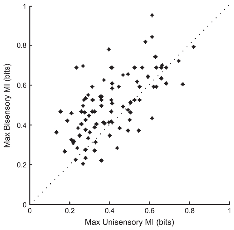
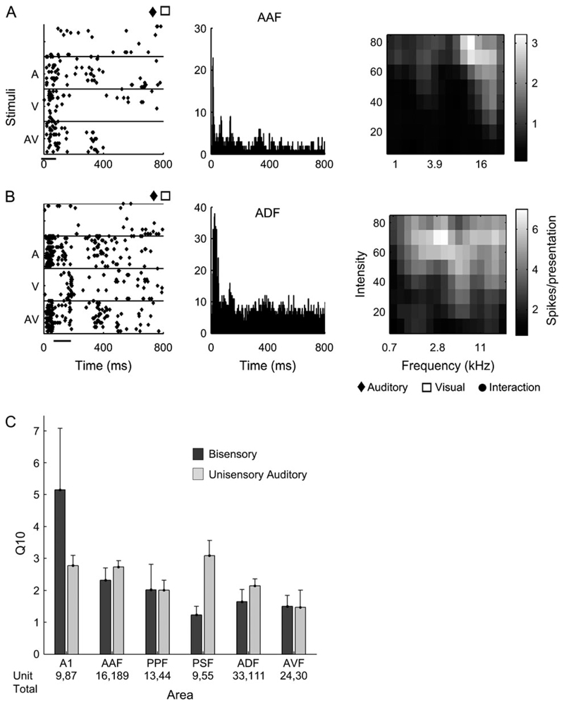
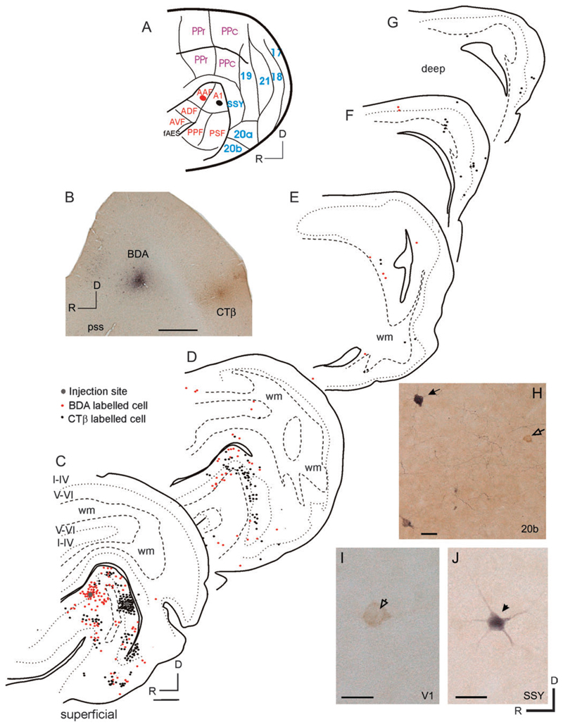
Recent studies, conducted almost exclusively in primates, have shown that several cortical areas usually associated with modality-specific sensory processing are subject to influences from other senses. Here we demonstrate using single-unit recordings and estimates of mutual information that visual stimuli can influence the activity of units in the auditory cortex of anesthetized ferrets. In many cases, these units were also acoustically responsive and frequently transmitted more information in their spike discharge patterns in response to paired visual-auditory stimulation than when either modality was presented by itself. For each stimulus, this information was conveyed by a combination of spike count and spike timing. Even in primary auditory areas (primary auditory cortex [A1] and anterior auditory field [AAF]), approximately 15% of recorded units were found to have nonauditory input. This proportion increased in the higher level fields that lie ventral to A1/AAF and was highest in the anterior ventral field, where nearly 50% of the units were found to be responsive to visual stimuli only and a further quarter to both visual and auditory stimuli. Within each field, the pure-tone response properties of neurons sensitive to visual stimuli did not differ in any systematic way from those of visually unresponsive neurons. Neural tracer injections revealed direct inputs from visual cortex into auditory cortex, indicating a potential source of origin for the visual responses. Primary visual cortex projects sparsely to A1, whereas higher visual areas innervate auditory areas in a field-specific manner. These data indicate that multisensory convergence and integration are features common to all auditory cortical areas but are especially prevalent in higher areas.

Figure 1

(A) Lateral view of the ferret brain showing the major sulci and gyri. (B) Sensory cortical areas in the ferret. The locations of known auditory, visual, somatosensory, and posterior parietal fields are indicated (Manger et al. 2002, 2004, 2005; Ramsay and Meredith 2004; Bizley et al. 2005). ASG, anterior sigmoid gyrus; as, ansinate sulcus; cns, coronal sulcus; crs, cruciate sulcus; LG, lateral gyrus; ls, lateral sulcus; OB, olfactory bulb; OBG, orbital gyrus; prs, presylvian sulcus; PSG, posterior sigmoid gyrus; pss, pseudosylvian sulcus; SSG, suprasylvian gyrus, sss, suprasylvian sulcus; A1, primary auditory cortex; AAF, anterior auditory field; PPF, posterior pseudosylvian field; PSF, posterior suprasylvian field; ADF, anterior dorsal field; AVF, anterior ventral field. fAES, anterior ectosylvian sulcal field; PPr, rostral posterior parietal cortex; 3b, primary somatosensory cortex; S2, secondary somatosensory cortex; S3, tertiary somatosensory cortex; D, dorsal; R, rostral. Scale bar is 5 mm in (A) 1 mm in (B).

Figure 2

Raster plots showing the range of response types recorded in auditory cortex. Responses of single units to broadband noise (A), a diffuse light flash (V) and combined auditory-visual stimulation (AV) are shown. (A) Example of a robust auditory response. (B, C) Units that responded to both stimuli presented separately. (D) Unit that responded only to visual stimulation. (E, F) Units that showed a clear enhancement of their unisensory responses when combined visual-auditory stimulation was used. Symbols indicate significant responses defined using MI measures. Units (A, B, and F) were located in field PSF, (C, E) in ADF, and (D) in PPF.

Figure 3

Location of auditory (blue dots), visual (green triangles), and bisensory (red diamonds) units plotted across the surface of the auditory cortex in 2 different animals (A, B). Cortical field boundaries (derived from measurements of unit best frequency and other response properties) are indicated by dashed lines. Recordings made within the ventral bank of the suprasylvian sulcus are shown “unfolded,” as indicated by the dotted lines in (A). Superimposed symbols indicate that multiple units were recorded at one site or, more commonly, that recordings were made at several depths. The recordings shown in (A) were made with a 4 × 4 silicon probe configuration, whereas those in (B) were obtained with a single linear probe with 16 recording sites. Recording sites in (B) have been jittered so that symbols are not completely overlapping. (C) Proportions of units responsive to each stimulus modality in each field (data pooled from all 6 animals). The total number of units recorded in each field is indicated at the top of each column. Bisensory units have been subdivided into 2 categories: those in which there was a response to both modalities of unisensory stimulation and those in which only one modality of stimulation produced a significant response when the stimuli were presented in isolation, but the addition of the other stimulus modality significantly modulated the response to the effective stimulus.

Figure 4

First spike latencies of auditory (A) and visual responses (B) of the multisensory units (i.e., units with significant responses to each modality). These are plotted separately for the 6 auditory fields that have been described in the ferret (see Fig. 1). Box plots depict the interquartile range and the central bar indicates the median response with the location of the notch showing the distribution of values around this. Kruskal-Wallis tests revealed significant (P < 0.05) interareal latency differences for the visual responses only. Significant differences, analyzed using Tukey-Kramer post hoc tests, between the latencies in each area are indicated by the horizontal bars.

Figure 5

Visual receptive fields in auditory cortex. (A) Raster plot showing the response of a unit recorded in AAF to stationary light flashes from an LED at different stimulus directions. This unit did not respond to sound, but a neighboring unit recorded with the same electrode had a best frequency of 20 kHz. The visual spatial receptive field was restricted in both azimuth and elevation (data not shown for elevation, but responses at the best azimuth were strongest for positions on or below the horizon). (B) Azimuth response profile for a different unit, recorded in ADF, which was also tuned for visual stimulus location. This visual response was significantly modulated by simultaneous stimulation of the contralateral ear. (C) Azimuth response profiles for all 31/39 of the spatially tuned cells recorded. Normalized spike rate in response to the arm-mounted LED and a contralateral noise burst are plotted (gray). The auditory stimulus location was therefore constant, whereas the azimuthal angle of the visual stimulus alone was varied. The mean spatial receptive field is overlaid in black.

Figure 6

(A) Auditory and visual response thresholds for 31 units (filled circles), and visual thresholds for a further 21 visual units (crosses on the x axis indicate that these latter units were not responsive to acoustic stimulation). (B) Raster plot showing the response of a single unit recorded in AVF to auditory and visual stimuli of increasing intensity. These stimuli were presented in a randomly interleaved fashion and are shown with the earliest presentations of each intensity combination positioned above the later ones. Note the clear latency separation of the response to each stimulus, with the visual response having a much longer latency than the response to sound. Suprathreshold stimuli were presented at a fixed intensity in one modality, whereas the intensity of the other stimulus was varied, as indicated by the values to the left of the plot. This unit had a visual threshold of 0.5 cd/m² and an auditory threshold of 34 dB SPL.

Figure 7

Cross-modal interactions in auditory cortex. Data from the same units plotted in Figure 2 are replotted as spike rates ± standard error of mean (corrected for spontaneous firing) for each of the 3 stimulation conditions with the percentage of response modulation values calculated using equation (2). The response modulation value reflects the difference between the linear sum of the unisensory responses and the response to bisensory stimulation.

Figure 8

Magnitude of cross-modal interactions in auditory cortex. (A) Bar graph showing the distribution of response modulation values (from eq. 2) derived from a comparison of evoked spike counts with each stimulus condition for all bisensory units. (B) Modulation values calculated in the same way but using the MI values rather than spike counts.

Figure 9

Scatterplot comparing the MI values for the most effective unisensory condition and the bisensory condition for all units that responded to both stimulus modalities. Points above the line indicate that more information is transmitted in response to combined visual-auditory stimulation than in the unisensory condition.

Figure 10

Decomposing the stimulus-related information in the spike discharge patterns. (A) The MI (in bits) calculated from spike counts plotted against the MI value obtained using mean response latency for all units in which the relevant response was previously classified as significant. × denotes auditory responses, ∇ denotes visual responses, ◇ denotes responses to bisensory stimulation. (B) Example raster plot in which the MI obtained using mean response latency (0.44 bits for the bisensory condition) exceeded that obtained using spike counts (0.13 bits) alone.

Figure 11

Cross-modal interactions depend on the relative timing of the visual and auditory stimuli. (A) Raster plot showing how the response of a bisensory unit varied when the sound was delayed relative to the light or vice versa. Stimulus conditions: A, auditory stimulus alone; V, visual stimulus alone; AV, simultaneous light and sound; VdA, light delayed relative to sound; VAd, sound delayed relative to light. The vertical lines indicate stimulus onset timing (light gray for light, dark gray for sound). (B) Mean (±standard deviation) evoked spike count for the visual stimulus alone, auditory stimulus alone, and for bisensory stimulation with the sound delayed relative to the light. The spike count changed significantly (Kruskal-Wallis test, P = 0.003) across these conditions, and post hoc tests revealed that the values obtained with the light alone and with interstimulus intervals of 100 and 200 ms were significantly lower than the spike counts recorded in the other bisensory stimulus conditions.

Figure 12

(A, B) Two examples of FRAs recorded from bisensory units. The left column shows the raster plots in response to auditory, visual, and bisensory stimuli (same conventions as Fig. 2). The middle column shows the pooled PSTH for 3 repetitions of each of the pure-tone stimuli used to construct the FRAs, which are shown in the right column. (A) Unit recorded in AAF. (B) Unit recorded in ADF. (C) Histograms showing the distribution of Q10 values for unisensory auditory and bisensory units in each of the 6 cortical fields.

Figure 13

Cortical inputs to the MEG. (A) Schematic of the ferret brain showing the sensory and posterior parietal areas. Previously described visual areas are labeled in blue, parietal in purple, and auditory in red. The CTβ and BDA injection sites in the MEG are represented by the red and black regions, respectively. (B) Photomicrograph of a flattened tangential section of the ferret EG showing the injection sites. Deposits of tracer were made by iontophoresis into frequency-matched locations (best frequency, 7 kHz) in the caudal and rostral MEG. (C-G) Drawings of flattened tangential sections of the cortex, ordered from lateral (C) to medial (G). CTβ-labeled cells are shown in red and BDA-labeled cells in black. Every fifth section (50-lm thick) was examined, but, for the purpose of illustration, labeling from pairs of sections was collapsed onto single sections. wm, white matter. Dotted lines mark the limit between layers IV and V; dashed lines delimit the white matter. Scale bars, 1 mm. (H-J) Examples of retrogradely labeled cells in area 20 (H), area 17 (I), and area SSY (J). The open arrow illustrates a CTβ-labeled cell, the closed arrows show BDA-labeled cells. Terminal fields were also visible in these sections. Scale bars, 50 μm.

Figure 14

Cortical inputs to higher level auditory areas on the AEG and PEG. (A) Schematic of the ferret brain showing the sensory and posterior parietal areas (as in Fig. 13). The black circle represents an injection of BDA made by iontophoresis into the AEG, and the red circle represents the site of the CTβ injection in the PEG. (B, C) Photomicrographs of flattened tangential sections showing the injection sites in the AEG and PEG, respectively. (D-H) Drawings of flattened tangential sections of the cortex, ordered from lateral (D) to medial (H). CTβ-labeled cells are shown in red and BDA-labeled cells in black. Scale bars, 1 mm. The centers of the injection sites are illustrated by gray circles. (I, J) Examples of retrogradely labeled cells in area 20 and area SSY. Scale bars, 50 μm. Other details as in Figure 13.

Figure 15

Cortical inputs to higher level auditory areas on the AEG. (A) Schematic of the ferret brain showing the sensory and posterior parietal areas (as in Fig. 13). The location of the CTβ injection site in the AEG is shown in black. The vertical lines represent the rostrocaudal level of the coronal sections in (C-I). (B) Photomicrographs of a coronal section showing the injection site. Scale bar, 1 mm. (C-I) Drawings of coronal sections of the cortex, ordered from rostral (C) to caudal (I). CTβ-labeled cells are shown in black. (J, K) Examples of retrogradely labeled cells in PPc and area 21, respectively. HP, hippocampus. Scale bars, 50 μm.

References

1. Adams JC. Heavy metal intensification of DAB-based HRP reaction product. J Histochem Cytochem. 1981;29:775. - PubMed
1. Aitkin LM, Kenyon CE, Philpott P. The representation of the auditory and somatosensory systems in the external nucleus of the cat inferior colliculus. J Comp Neurol. 1981;196:25–40. - PubMed
1. Alitto HJ, Usrey WM. Influence of contrast on orientation and temporal frequency tuning in ferret primary visual cortex. J Neuro-physiol. 2004;91:2797–2808. - PubMed
1. Bajo VM, Nodal FR, Bizley JK, Moore DR, King AJ. The Ferret Auditory Cortex: Descending projections to the inferior colliculus. Cereb Cortex. 2006 doi: 10.1093/cercor/bhj164. - DOI - PMC - PubMed
1. Bell AH, Corneil BD, Munoz DP, Meredith MA. Engagement of visual fixation suppresses sensory responsiveness and multisensory integration in the primate superior colliculus. Eur J Neurosci. 2003;18:2867–2873. - PubMed
Publication types