Modification and optimization of the united-residue (UNRES) potential energy function for canonical simulations. I. Temperature dependence of the effective energy function and tests of the optimization method with single training proteins

Abstract

We report the modification and parametrization of the united-residue (UNRES) force field for energy-based protein structure prediction and protein folding simulations. We tested the approach on three training proteins separately: 1E0L (beta), 1GAB (alpha), and 1E0G (alpha + beta). Heretofore, the UNRES force field had been designed and parametrized to locate native-like structures of proteins as global minima of their effective potential energy surfaces, which largely neglected the conformational entropy because decoys composed of only lowest-energy conformations were used to optimize the force field. Recently, we developed a mesoscopic dynamics procedure for UNRES and applied it with success to simulate protein folding pathways. However, the force field turned out to be largely biased toward -helical structures in canonical simulations because the conformational entropy had been neglected in the parametrization. We applied the hierarchical optimization method, developed in our earlier work, to optimize the force field; in this method, the conformational space of a training protein is divided into levels, each corresponding to a certain degree of native-likeness. The levels are ordered according to increasing native-likeness; level 0 corresponds to structures with no native-like elements, and the highest level corresponds to the fully native-like structures. The aim of optimization is to achieve the order of the free energies of levels, decreasing as their native-likeness increases. The procedure is iterative, and decoys of the training protein(s) generated with the energy function parameters of the preceding iteration are used to optimize the force field in a current iteration. We applied the multiplexing replica-exchange molecular dynamics (MREMD) method, recently implemented in UNRES, to generate decoys; with this modification, conformational entropy is taken into account. Moreover, we optimized the free-energy gaps between levels at temperatures corresponding to a predominance of folded or unfolded structures, as well as to structures at the putative folding-transition temperature, changing the sign of the gaps at the transition temperature. This enabled us to obtain force fields characterized by a single peak in the heat capacity at the transition temperature. Furthermore, we introduced temperature dependence to the UNRES force field; this is consistent with the fact that it is a free-energy and not a potential energy function. beta

Fig. 1

The UNRES model of the polypeptide chain. Dark circles represent united peptide groups (p), open circles represent the C^α atoms, which serve as geometric points. Ellipsoids represent side chains, with their centers of mass at the SC’s. The p’s are located half-way between two consecutive C^α atoms. The virtual-bond angles θ, the virtual-bond dihedral angles γ, and the angles α_SC and β_SC that define the location of a side chain with respect to the backbone are also indicated.

Fig. 2

Schematic plots of the variation of the free energy (lower panels), energy (upper panels, solid lines), and heat capacity (upper panels, dashed lines) of models of three protein systems (a, b, and c) with three hierarchy levels: 0 (non-native), 1 (intermediate), and 2 (native); (a) with the free energies of all three levels intersecting at the folding-transition temperatures, (b) intersecting at different but close temperatures and (c) intersecting at significantly different temperatures. The horizontal lines in the upper panels are the energies of conformations at level 0 (dot-dashed lines), level 1 (dotted lines), and level 2 (dash-double-dotted lines); the straight lines in the lower panels with line styles as above, show the variation of the free energies of each of the levels with temperatures. For clarity, the energies of the individual levels are assumed to be independent of temperature (i.e., all microstates of the same level have the same energy) in the range of temperatures considered. When the free-energy curves of the levels intersect at exactly the same temperature (a), the heat-capacity peak is sharp; it becomes broader when the points of intersection diverge (b), to split, finally, into two separate peaks when the difference between the intersection points becomes large (c). All units are arbitrary and, therefore, no scale is shown on the axes.

Fig. 3

Illustration of the role of inclusion of the Shannon-entropy term in eq 25 in the last iteration of the optimization of the force field using 1GAB as the training protein (section 4.2). Left panels: linear plots of the dimensionless free energies (U/RT − ln ω) at T = 300 K (with ω defined by eq 15) of the conformations of the 1GAB protein at level 0 (filled circles), 1 (filled diamonds), 2 (filled triangles), and 3 (asterisks); the symbols are seen most clearly in panel b. Only the low-free-energy parts are shown for clarity, and the F/RT span is the same on all three panels for better comparison. Right panels: plots of partial dimensionless free energies calculated by taking only the N lowest-free-energy conformations (where N is the variable of the abscissa) sorted according to U/RT − ln ω. Solid lines: level 0; short-dashed lines: level 1; long-dashed lines: level 2; dash-dotted lines: level 3. (a) Before minimizing the target function, (b) After minimizing the target function without including the Shannon-entropy term. (c) After minimizing the target function with inclusion of the Shannon-entropy term.

Fig. 4

The experimental structures of (a) 1E0L, (b) 1GAB, and (c) 1E0G. The native-like elements considered in the hierarchical optimization are both color-coded and marked with symbols used in the text. For 1E0L, the part of the chain shared by β₁ and β₂ is colored yellow. The MOLMOL software has been used to draw the pictures.

Fig. 5

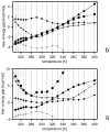
Variation of the free-energy gaps (ΔF) between level 0 and 1 (solid lines and filled circles) and levels 1 and 2 (dashed lines and filled diamonds) in optimization of the UNRES force field starting from the F2 force field of ref . The gaps at the temperatures included in the target function (eq 25) are shown as filled symbols and the temperatures are marked with thin dotted vertical lines, (a) Initial gaps, (b) gaps after iteration 1, (c) gaps after iteration 2.

Fig. 6

Variation of the dimensionless free energy (F/RT) of the 1E0L protein with q at selected temperatures in consecutive iterations of the optimization of the UNRES force field starting from the F2 force field of ref . (a) Initial, (b) after iteration 1, (c) after iteration 2.

Fig. 7

Superposition of the 10 most probable structures of 1E0L calculated by using the MREMD method with the F2 force field at T = 300 K (a) and T = 500 K (b). The C-terminus is marked for tracing purposes. The MOLMOL software has been used to draw the pictures.

Fig. 8

The experimental structure of 1E0L (a) and three most probable structures obtained with the final force field optimized starting from the F2 force field (b–d) at T = 600 K. The C^α atoms of the residues involved in the N-terminal γ-turn and the C-terminal β-turn in the native structures are shown as gray spheres. It can be seen that the C-terminal β-turn is shifted or distorted and the C-terminal segment is a part of the β-hairpin in the calculated structures as opposed to the experimental structure; this results in large RMSD values although the topology of the calculated structures is native-like. The N-terminus is marked for tracing purposes. The MOLMOL software has been used to draw the pictures.

Fig. 9

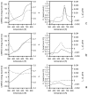
Left panels: plots of the energy (eq 20; solid lines) and q (dashed lines); right panels: plots of the heat capacity (eq 21; solid lines) and dq/dT (dashed lines) of the 1E0L protein in consecutive iterations of optimization of the UNRES force field starting from the F2 force field of ref . (a) Initial curves, (b) iteration 1, (c) iteration 2.

Fig. 10

Left panel: a plot of the energy (eq 20; solid line) and q (dashed line); right panel: a plot of the heat capacity (eq 21); solid line) and dq/dT (dashed line) for the 1E0L protein, corresponding to the UNRES force field optimized by starting from the scaled 4P force field of ref .

Fig. 11

Variation of the free-energy gaps between level 0 and 1 (solid lines and filled circles) 1 and 2 (short-dashed lines and filled diamonds), and 2 and 3 (long-dashed lines and filled triangles) in optimization of the UNRES force field for the 1GAB protein starting from the 4P force field developed in ref . The gaps at the temperatures included in the target function (eq 25) are shown as filled symbols and the temperatures are marked with thin dotted vertical lines, (a) Initial gaps calculated with temperature-independent force field (eq 1), (b) gaps after iteration 3 of the optimization of the temperature-independent force field, (c) initial gaps calculated with energy-term weights corresponding to panel (b) and column interim1 of Table but with temperature-dependent force field (eq 5), (d) gaps calculated with temperature-dependent force field with only energy-term weights optimized, (e) gaps calculated with temperature-dependent force field with energy-term weights and well-depths of the U_SCiSCj potentials optimized.

Fig. 11

Variation of the free-energy gaps between level 0 and 1 (solid lines and filled circles) 1 and 2 (short-dashed lines and filled diamonds), and 2 and 3 (long-dashed lines and filled triangles) in optimization of the UNRES force field for the 1GAB protein starting from the 4P force field developed in ref . The gaps at the temperatures included in the target function (eq 25) are shown as filled symbols and the temperatures are marked with thin dotted vertical lines, (a) Initial gaps calculated with temperature-independent force field (eq 1), (b) gaps after iteration 3 of the optimization of the temperature-independent force field, (c) initial gaps calculated with energy-term weights corresponding to panel (b) and column interim1 of Table but with temperature-dependent force field (eq 5), (d) gaps calculated with temperature-dependent force field with only energy-term weights optimized, (e) gaps calculated with temperature-dependent force field with energy-term weights and well-depths of the U_SCiSCj potentials optimized.

Fig. 12

Left panels: plots of the energy (solid lines) and q (dashed lines), right panels: plots of the heat capacity (solid lines) and dq/dT (dashed lines) of the 1GAB protein in consecutive iterations of the optimization of the UNRES force field. (a) Plots corresponding to the temperature-independent force field and initial parameters, (b) optimized temperature-independent force field after three iterations, (c) energy-term weights determined in part (b) used as initial ones in a temperature-dependent force field, (d) temperature-dependent force field with only energy-term weights optimized, (e) temperature-dependent force field with energy-term weights and well-depths of the U_SCiSCj potentials optimized.

Fig. 12

Left panels: plots of the energy (solid lines) and q (dashed lines), right panels: plots of the heat capacity (solid lines) and dq/dT (dashed lines) of the 1GAB protein in consecutive iterations of the optimization of the UNRES force field. (a) Plots corresponding to the temperature-independent force field and initial parameters, (b) optimized temperature-independent force field after three iterations, (c) energy-term weights determined in part (b) used as initial ones in a temperature-dependent force field, (d) temperature-dependent force field with only energy-term weights optimized, (e) temperature-dependent force field with energy-term weights and well-depths of the U_SCiSCj potentials optimized.

Fig. 13

Stereo view of the C^α-trace of the experimental structure of 1GAB (gray sticks) and the ten most probable structures of 1GAB calculated at T = 280 K with the force field optimized on that protein (black lines). The N-terminus is marked for tracing purposes. The RMSD from the native structure averaged over the entire ensemble at T = 280 K is equal to 4.1 Å. The MOLMOL software has been used to draw the pictures.

Fig. 14

Plots of (a) heat capacity and (b) q calculated using consecutive 2,000,000 MD step/trajectory windows taken from the MREMD run of 1GAB with the optimized force field and variation of log N, (c) the decimal logarithm of the numbers of conformations (N) belonging to consecutive hierarchy levels and (d) free-energy gaps at T = 290 K with the duration of simulation. The curves in panels (a) and (b) are colored according to the duration of simulation, the color scale (in million steps) being shown above panel (b). In (c) the solid line corresponds to level 0, short-dashed line to level 1, long-dashed line to level 2, and dotted line to level 3 (native). In (d) the solid line corresponds to the gap between levels 0 and 1, short-dashed line to the gap between levels 1 and 2, and long-dashed line to the gap between levels 2 and 3.

Fig. 14

Plots of (a) heat capacity and (b) q calculated using consecutive 2,000,000 MD step/trajectory windows taken from the MREMD run of 1GAB with the optimized force field and variation of log N, (c) the decimal logarithm of the numbers of conformations (N) belonging to consecutive hierarchy levels and (d) free-energy gaps at T = 290 K with the duration of simulation. The curves in panels (a) and (b) are colored according to the duration of simulation, the color scale (in million steps) being shown above panel (b). In (c) the solid line corresponds to level 0, short-dashed line to level 1, long-dashed line to level 2, and dotted line to level 3 (native). In (d) the solid line corresponds to the gap between levels 0 and 1, short-dashed line to the gap between levels 1 and 2, and long-dashed line to the gap between levels 2 and 3.

Fig. 15

Variation of initial (a) and final (b) free-energy gaps with temperature in the optimization of the UNRES force field using 1E0G as a training protein. The gaps at the temperatures included in the target function (eq 25) are shown as filled symbols and the temperatures are marked with thin dotted vertical lines. Dotted lines and asterisks: gaps between level -1 (“anti-native”) and sum of other levels; solid lines and filled circles: gaps between level 0 and sum of levels 1 and 2; short-dashed lines and filled diamonds: gaps between level 1 and 2; long-dashed lines and filled triangles: gaps between level 2 and 3; dash-dotted lines and filled squares: gaps between levels 3 and 4.

Fig. 16

Left panels: plots of the energy (solid lines) and q (dashed lines); right panels: plots of the heat capacity (solid lines) and dq/dT (dashed lines) for the 1E0G protein before (a) and after (b) optimization of the UNRES force field.

Fig. 17

Stereo view of the C^α-trace of the experimental structure of 1E0G (gray sticks) and ten most probable structures of 1E0G calculated at T = 280 K with the force field optimized on that protein (black lines). The N-terminus is marked for tracing purposes The RMSD from the native structure averaged over the entire ensemble at T = 280 K is equal to 5.5 Å. The MOLMOL software has been used to draw the pictures.

Fig. 18

Plots of (a) heat capacity and (b) q calculated using 2,000,000 MD step/trajectory windows taken from the MREMD run of 1E0G with the optimized force field, and (c) variation of log N, the decimal logarithm of numbers of conformations belonging to consecutive hierarchy levels and (d) free-energy gaps at T = 290 K with the duration of simulation. The curves in panels (a) and (b) are colored according to the duration of simulation, the color scale (in million steps) being shown above panel (b). In (c) the dotted line corresponds to level -1 (anti-native), solid line to level 0, short-dashed line to level 1, long-dashed line to level 2, dot-dashed line to level 3, and dot-double-dashed line to level 4 (native). In (d) the solid line corresponds to the gap between levels 0 and the sum of levels 1 and 2, short-dashed line to the gap between levels 1 and 2, long-dashed line to the gap between levels 2 and 3 and dot-dashed line to the gap between levels 3 and 4.

Fig. 18

Plots of (a) heat capacity and (b) q calculated using 2,000,000 MD step/trajectory windows taken from the MREMD run of 1E0G with the optimized force field, and (c) variation of log N, the decimal logarithm of numbers of conformations belonging to consecutive hierarchy levels and (d) free-energy gaps at T = 290 K with the duration of simulation. The curves in panels (a) and (b) are colored according to the duration of simulation, the color scale (in million steps) being shown above panel (b). In (c) the dotted line corresponds to level -1 (anti-native), solid line to level 0, short-dashed line to level 1, long-dashed line to level 2, dot-dashed line to level 3, and dot-double-dashed line to level 4 (native). In (d) the solid line corresponds to the gap between levels 0 and the sum of levels 1 and 2, short-dashed line to the gap between levels 1 and 2, long-dashed line to the gap between levels 2 and 3 and dot-dashed line to the gap between levels 3 and 4.

Fig. 19

Stereo views of the C^α traces of the representatives of the most probable (upper panels) and the native-like (lower panels) clusters of the conformations of the proteins used to test the force field derived on 1GAB. The representatives of the native-like clusters (thin black sticks) are superposed on the experimental structures (thick gray sticks). See Table 8 for RMSD values and probabilities. The MOLMOL software has been used to draw the pictures. (a) 1BDD (the most probable cluster is the native-like cluster and therefore only one picture is shown; (b) 1LQ7; (c) 1E68; (d) 1CLB; (e) 1P68; (f) 1POU; (g) 1PRU; (h) 1KOY. The MOLMOL software has been used to draw the pictures.

Fig. 19

Stereo views of the C^α traces of the representatives of the most probable (upper panels) and the native-like (lower panels) clusters of the conformations of the proteins used to test the force field derived on 1GAB. The representatives of the native-like clusters (thin black sticks) are superposed on the experimental structures (thick gray sticks). See Table 8 for RMSD values and probabilities. The MOLMOL software has been used to draw the pictures. (a) 1BDD (the most probable cluster is the native-like cluster and therefore only one picture is shown; (b) 1LQ7; (c) 1E68; (d) 1CLB; (e) 1P68; (f) 1POU; (g) 1PRU; (h) 1KOY. The MOLMOL software has been used to draw the pictures.

Fig. 19

Stereo views of the C^α traces of the representatives of the most probable (upper panels) and the native-like (lower panels) clusters of the conformations of the proteins used to test the force field derived on 1GAB. The representatives of the native-like clusters (thin black sticks) are superposed on the experimental structures (thick gray sticks). See Table 8 for RMSD values and probabilities. The MOLMOL software has been used to draw the pictures. (a) 1BDD (the most probable cluster is the native-like cluster and therefore only one picture is shown; (b) 1LQ7; (c) 1E68; (d) 1CLB; (e) 1P68; (f) 1POU; (g) 1PRU; (h) 1KOY. The MOLMOL software has been used to draw the pictures.

References

1. Skolnick J, Zhang Y, Arakaki AK, Kolińsi A, Boniecki M, Szilagyi A, Kihara D. Proteins: Struct Func Genet. 2003;53:469. - PubMed
1. Eskow E, Bader D, Byrd R, Crivelli S, Head-Gordon T, Lamberti V, Schnabel R. Math Program. 2004;101:497.
1. Fujitsuka Y, Takada S, Luthey-Schulten ZA, Wolynes PG. Proteins: Struct Func Genet. 2004;54:88. - PubMed
1. Scheraga HA, Liwo A, Ołdziej S, Czaplewski C, Pillardy J, Ripoll DR, Vila JA, KaŸmierkiewicz R, Saunders JA, Arnautova YA, Jagielska A, Chinchio M, Nanias M. Frontiers in Bioscience. 2004;9:3296. - PubMed
1. Petrey D, Honig B. Mol Cell. 2005;20:811. - PubMed
Publication types